Classification and Regression Trees (CART)
History of Decision Trees
late 1970s - J Ross Quinlan : ID3 (Iterative Dichotomizer)
early 1980s - EB Hunt, J Marinm PT Stone: C4.5 (a successpr of ID3)
1084 - L. Breiman, J. Friedman, R Olshen, C. Stone: CART (Classification and Regression Trees)
Model
\[Y = f(X_1, X_2,... X_n) + \epsilon\] Goal: What is \(f\)?
How do we estimate \(f\) ?
Data-driven methods:
estimate \(f\) using observed data without making explicit assumptions about the functional form of \(f\).
Parametric methods:
estimate \(f\) using observed data by making assumptions about the functional form of \(f\).
Errors
Reducible error
Irreducible error
General Process of Classification and Regression
In-class diagram
Classification and Regression Trees
Classification tree - Outcome is categorical
Regression tree - Outcome is numeric
Classification and Regression Trees
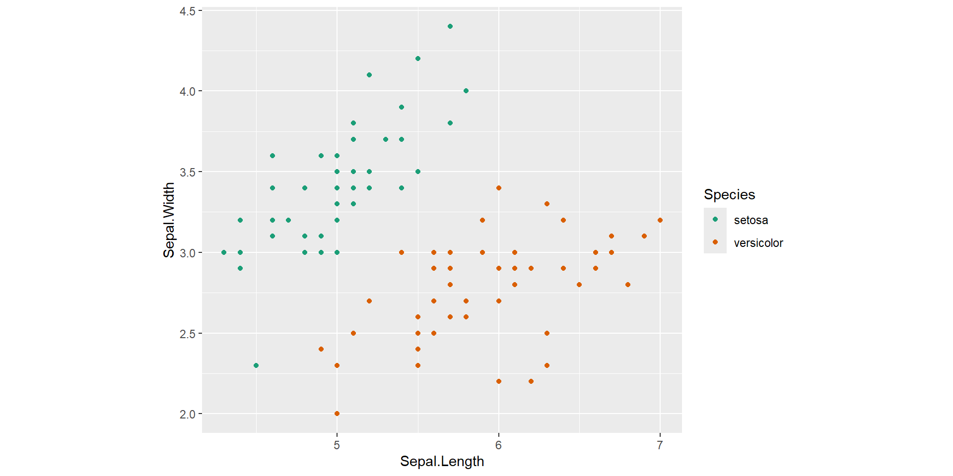
CART models work by partitioning the feature space into a number of simple rectangular regions, divided up by axis parallel splits.
The splits are logical rules that split feature-space into two non-overlapping subregions.
Example: Feature space
Features: Sepal Length, Sepal Width
Outcome: setosa/versicolor
![]()
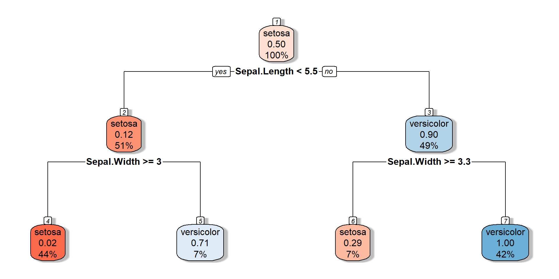
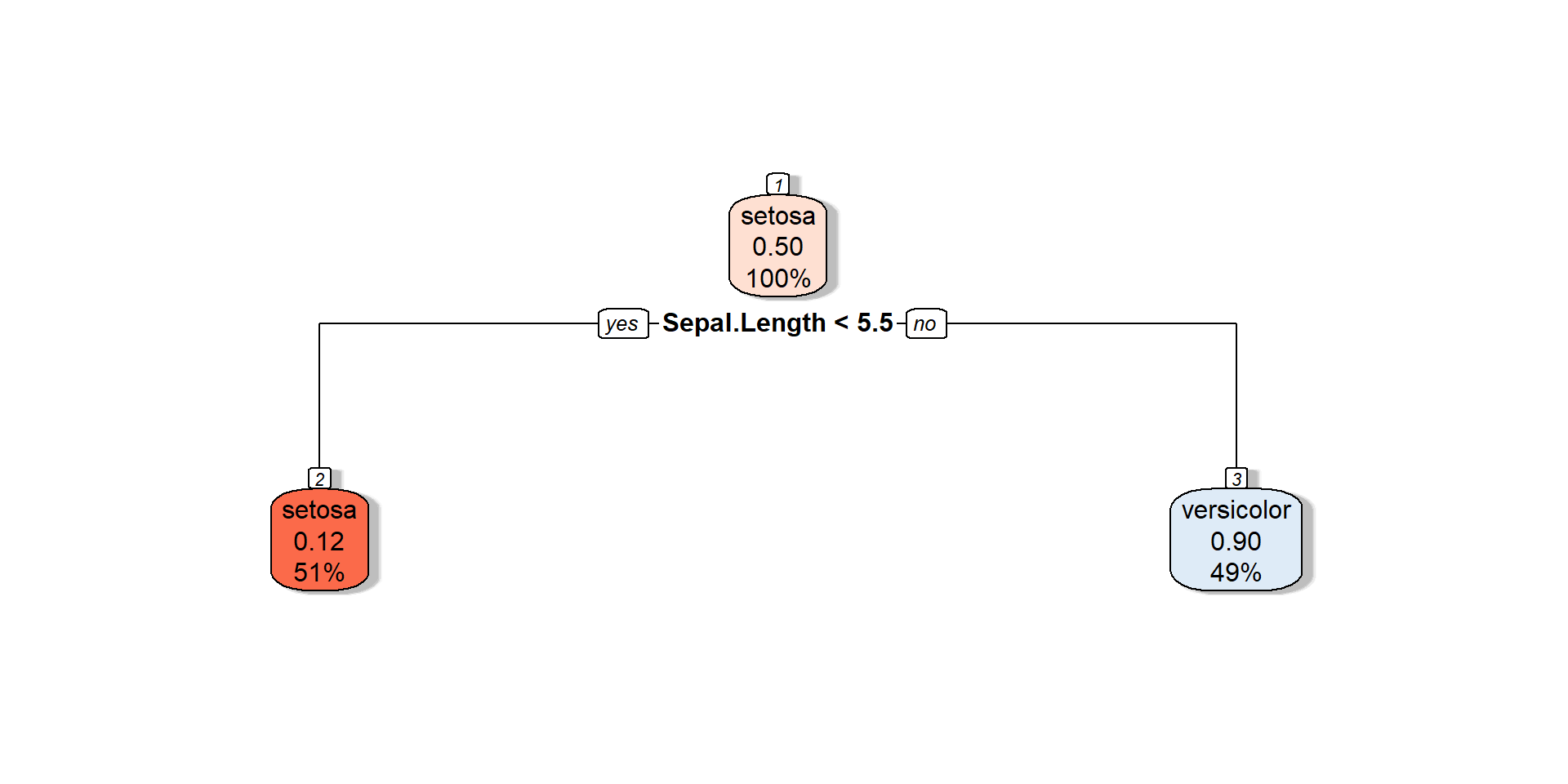
Decision tree
![]()
n= 100

node), split, n, loss, yval, (yprob)
      * denotes terminal node

1) root 100 50 setosa (0.50000000 0.50000000)
  2) Sepal.Length< 5.45 51  6 setosa (0.88235294 0.11764706)
    4) Sepal.Width>=2.95 44  1 setosa (0.97727273 0.02272727) *
    5) Sepal.Width< 2.95 7  2 versicolor (0.28571429 0.71428571) *
  3) Sepal.Length>=5.45 49  5 versicolor (0.10204082 0.89795918)
    6) Sepal.Width>=3.25 7  2 setosa (0.71428571 0.28571429) *
    7) Sepal.Width< 3.25 42  0 versicolor (0.00000000 1.00000000) *
Decision tree
![]()
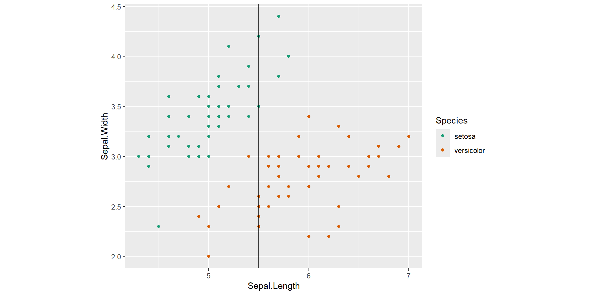
Root node split
![]()
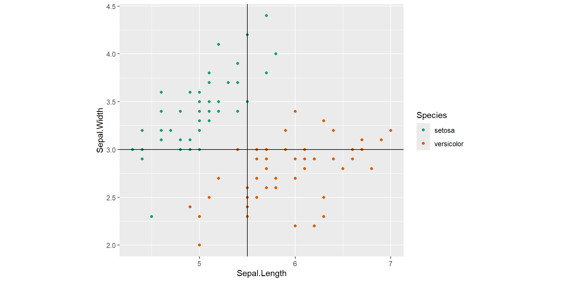
Root node split, Decision node split - right
![]()
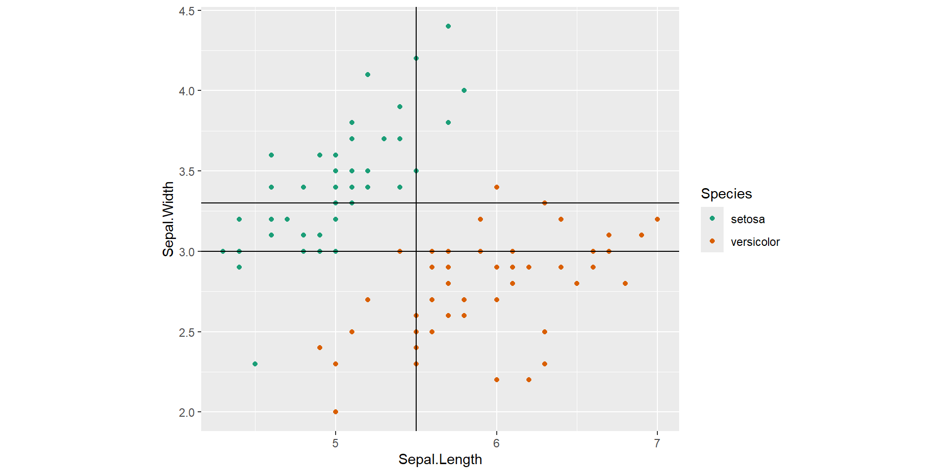
Root node split, Decision node splits
![]()
Shallow decision tree
![]()
Two key ideas underlying trees
Recursive partitioning (for constructing the tree)
Pruning (for cutting the tree back)
Pruning is a useful strategy for avoiding over fitting.
There are some alternative methods to avoid over fitting as well.
Constructing Classification Trees
Recursive Partitioning
Main questions
Splitting variable
Which attribute/ feature should be placed at the root node?
Which features will act as internal nodes?
Splitting point
Looking for a split that increases the homogeneity (or “pure” as possible) of the resulting subsets.
Example
split that increases the homogeneity
![]()
Example (cont.)
split that increases the homogeneity .
![]()
Key idea
Iteratively split variables into groups
Evaluate “homogeneity” within each group
Split again if necessary
How does a decision tree determine the best split?
Decision tree uses entropy and information gain to select a feature which gives the best split.
Gini index
Gini index for rectangle \(A\) is defined by
\[I(A) = 1- \sum_{k=1}^mp_k^2\]
\(p_k\) - proportion of records in rectangle \(A\) that belong to class \(k\)
- Gini index takes value 0 when all the records belong to the same class.
Gini index (cont)
In the two-class case Gini index is at peak when \(p_k = 0.5\)
Entropy measure
\[entropy(A) = - \sum_{k=1}^{m}p_k log_2(p_k)\]
Example:
![]()
Finding the best threshold split?
In-class demonstration
Overfitting in decision trees
Overfitting refers to the condition when the model completely fits the training data but fails to generalize the testing unseen data.
If a decision tree is fully grown or when you increase the depth of the decision tree, it may lose some generalization capability.
Pruning is a technique that is used to reduce overfitting. Pruning simplifies a decision tree by removing the weakest rules.
Stopping criteria
Tree depth (number of splits)
Minimum number of records in a terminal node
Minimum reduction in impurity
Complexity parameter (\(CP\) ) - available in rpart package
Pre-pruning (early stopping)
max_depth
min_samples_leaf
min_samples_split
Post pruning
Simplify the tree after the learning algorithm terminates
The idea here is to allow the decision tree to grow fully and observe the CP value
Simplify the tree after the learning algorithm terminates
- Complexity of tree is measured by number of leaves.
\(L(T) = \text{number of leaf nodes}\)
The more leaf nodes you have, the more complexity.
We need a balance between complexity and predictive power
Total cost = measure of fit + measure of complexity
Total cost = measure of fit + measure of complexity
measure of fit: error
measure of complexity: number of leaf nodes (\(L(T)\))
\(\text{Total cost } (C(T)) = Error(T) + \lambda L(T)\)
The parameter \(\lambda\) trade off between complexity and predictive power. The parameter \(\lambda\) is a penalty factor for tree size.
\(\lambda = 0\): Fully grown decision tree
\(\lambda = \infty\): Root node only
\(\lambda\) between 0 and \(\infty\) balance predictive power and complexity.
Example: candidate for pruning (in-class)
![]()
Classification trees - label of terminal node
![]()
labels are based on majority votes.
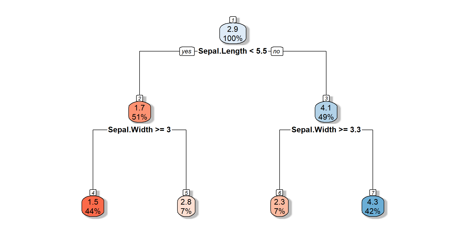
Regression Trees
![]()
Regression Trees
Value of the terminal node: average outcome value of the training records that were in that terminal node.
Your turn: Impurity measures for regression tree
Decision trees - advantages
Decision trees - disadvantages


