| Predicted | Positive | Negative |
|---|---|---|
| Positive | A - TP | B-FP |
| Negative | C - FN | D-TN |
Measuring Performance
Department of Statistics, Faculty of Applied Sciences
University of Sri Jayewardenepura, Sri Lanka
Measures for Regression
Loss function
- Function that calculates loss for a single data point
\(e_i = y_i - \hat{y_i}\)
\(e_i^2 = (y_i - \hat{y_i})^2\)
Cost function
- Calculates loss for the entire data sets
\[ME = \frac{1}{n}\sum_{i=1}^n e_i\]
Numeric outcome: Evaluations
Prediction accuracy measures (cost functions)
Mean Error
\[ME = \frac{1}{n}\sum_{i=1}^n e_i\]
- Error can be both negative and positive. So they can cancel each other during the summation.
Mean Absolute Error (L1 loss)
\[MAE = \frac{1}{n}\sum_{i=1}^n |e_i|\]
Mean Squared Error (L2 loss)
\[MSE = \frac{1}{n}\sum_{i=1}^n e^2_i\]
Mean Percentage Error
\[MPE = \frac{1}{n}\sum_{i=1}^n \frac{e_i}{y_i}\]
Mean Absolute Percentage Error
\[MAPE = \frac{1}{n}\sum_{i=1}^n |\frac{e_i}{y_i}|\]
Root Mean Squared Error
\[RMSE = \sqrt{\frac{1}{n}\sum_{i=1}^n e^2_i}\]
Visualizaion of error distribution
Graphical representations reveal more than metrics alone.
Accuracy Measures on Training Set vs Test Set
Accuracy measure on training set: Tells about the model fit
Accuracy measure on test set: Model ability to predict new data
Evaluate Classifier Against Benchmark
Naive approach: approach relies soley on \(Y\)
Outcome: Numeric
Naive Benchmark: Average (\(\bar{Y}\))
A good prediction model should outperform the benchmark criterion in terms of predictive accuracy.
Measures for predicted classes
Confusion matrix/ Classification matrix
TP - True Positive
FP - False Positive
FN - False Negative
TN - True Negative
\(A\) - True Positive
\(B\) - False Positive
\(C\) - False Negative
\(D\) - True Negative
\[Sensitivity = \frac{A}{A+C}\]
\[Specificity = \frac{D}{B+D}\]
\[Prevalence = \frac{A+C}{A+B+C+D}\]
\[\text{Detection Rate} = \frac{A}{A+B+C+D}\]
\[\text{Detection Prevalence} = \frac{A+B}{A+B+C+D}\]
\[\text{Balance Accuracy}=\frac{Sensitivity + Specificity}{2}\]
\[Precision = \frac{A}{A+B}\]
\[Recall = \frac{A}{A+C}\]
F-1 score
\[F_1 = \frac{2 \times (\text{precision} \times \text{recall})}{\text{precision + recall}}\] The \(F1\) score can be interpreted as a harmonic mean of the precision and recall, where an \(F1\) score reaches its best value at 1 and worst score at 0. The relative contribution of precision and recall to the F1 score are equal.
F-beta score
\[F_1 = \frac{(1+\beta^2) \times (\text{precision} \times \text{recall})}{(\beta^2 \times \text{precision}) + \text{recall}}\]
Weighted harmonic mean of the precision and recall, reaching its optimal value at 1 and worst value at 0.
The beta parameter determines the weight of recall in the combined score.
\[\beta < 1 - \text{more weight to precision }\]
\[\beta > 1 - \text{favors recall}\]
Positive Prediction Value (PPV)
\[PPV = \frac{sensitivity \times prevalence}{(sensitivity \times prevalence)+((1-specificity)\times (1-prevalence))}\]
Negative Prediction Value (PPV)
\[NPV = \frac{specificity \times (1-prevalence)}{( (1-sensitivity) \times prevalence)+(specificity \times (1-prevalence))}\]
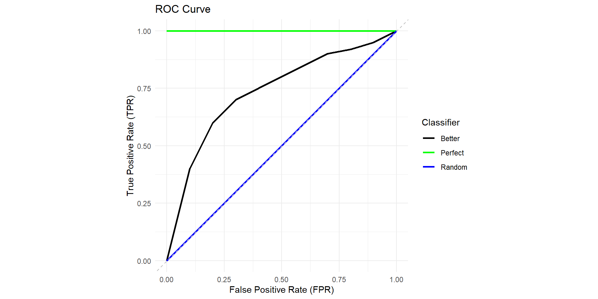
Receiver Operating Characteristic (ROC) curve

\[TPR = \frac{TP}{TP+FN}\]
\[FPR = \frac{FP}{FP+TN}\]
Area Under Curve (AUC)
Perfect classifier: \(AUC = 1\)
Random classifier: \(AUC = 0.5\)