Time Series Forecasting with Python: Method 1

Loading packages

import pandas as pd
import plotnine as p9 
from plotnine import *
from plotnine.data import *
import numpy as np

Read data

airpassenger = pd.read_csv('AirPassengers.csv')
airpassenger['Month']= pd.to_datetime(airpassenger['Month'])

Visualise data

ggplot(airpassenger, aes(x='Month', y='#Passengers'))+geom_line()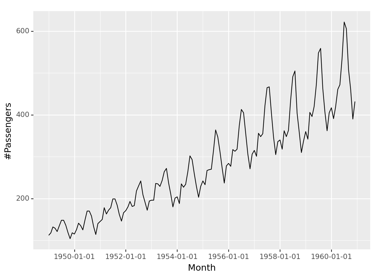

Training set vs Test set

# Define training and test separation point
split_date = '1960-01'

# Visualize data
g = (
    ggplot(airpassenger, aes(x='Month', y='#Passengers')) +
    geom_line(color='blue') +
    geom_vline(xintercept=pd.to_datetime(split_date), linetype='dashed', color='red') +
    labs(
        title='Air Passenger Counts Over Time',
        x='Month',
        y='Number of Passengers'
    ) +
    theme_minimal()
)

# Print plot
print(g)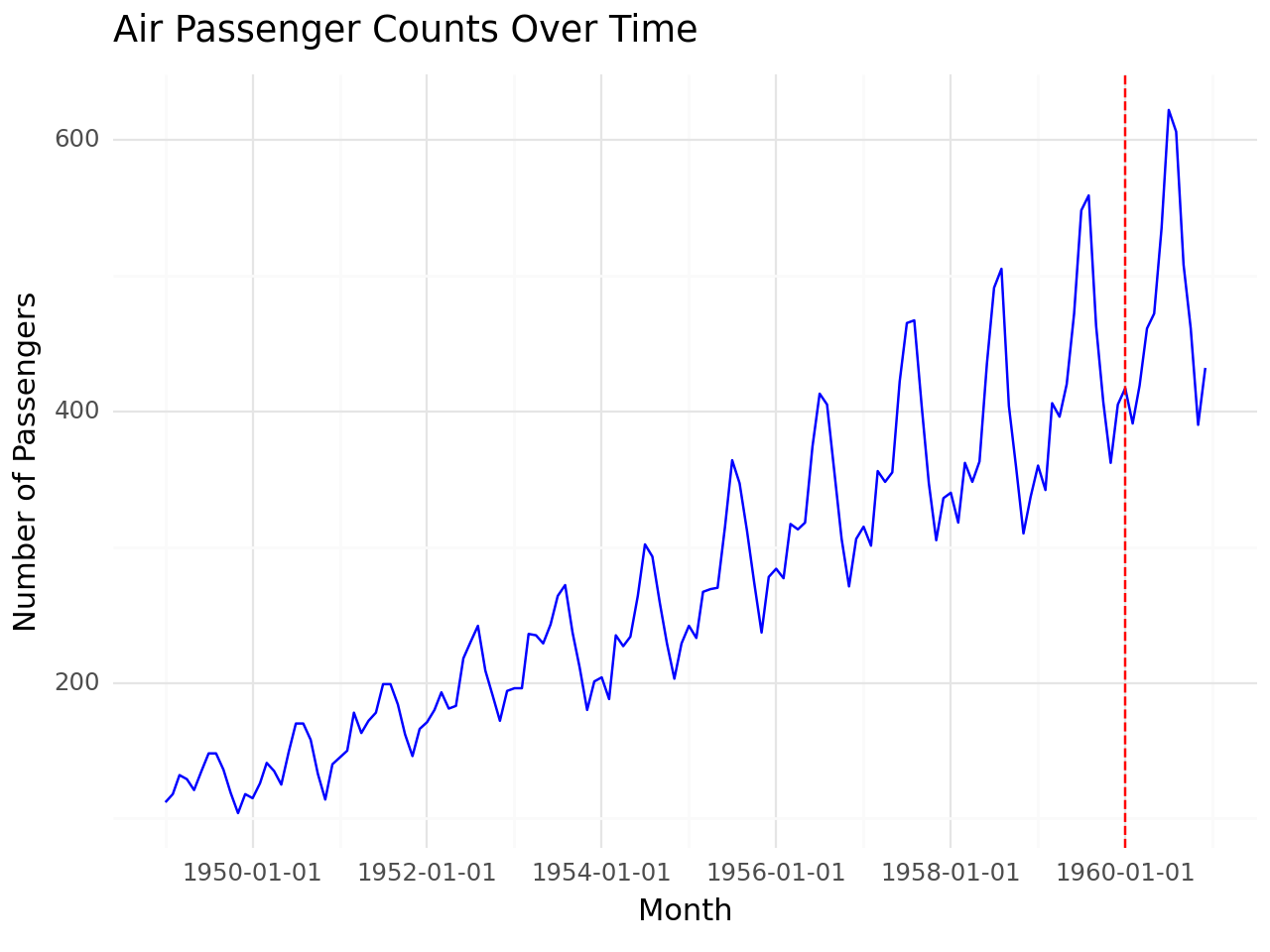

Apply log transformation

airpassenger['Log_Passengers'] = np.log(airpassenger['#Passengers'])

# Define training and test separation point
split_date = '1960-01-01'

# Visualize data
g = (
    ggplot(airpassenger, aes(x='Month', y='Log_Passengers')) +
    geom_line(color='blue') +
    geom_vline(xintercept=pd.to_datetime(split_date), linetype='dashed', color='red') +
    labs(
        title='Log-Transformed Air Passenger Counts Over Time',
        x='Month',
        y='Log(Number of Passengers)'
    ) +
    theme_minimal()
)

# Print plot
print(g)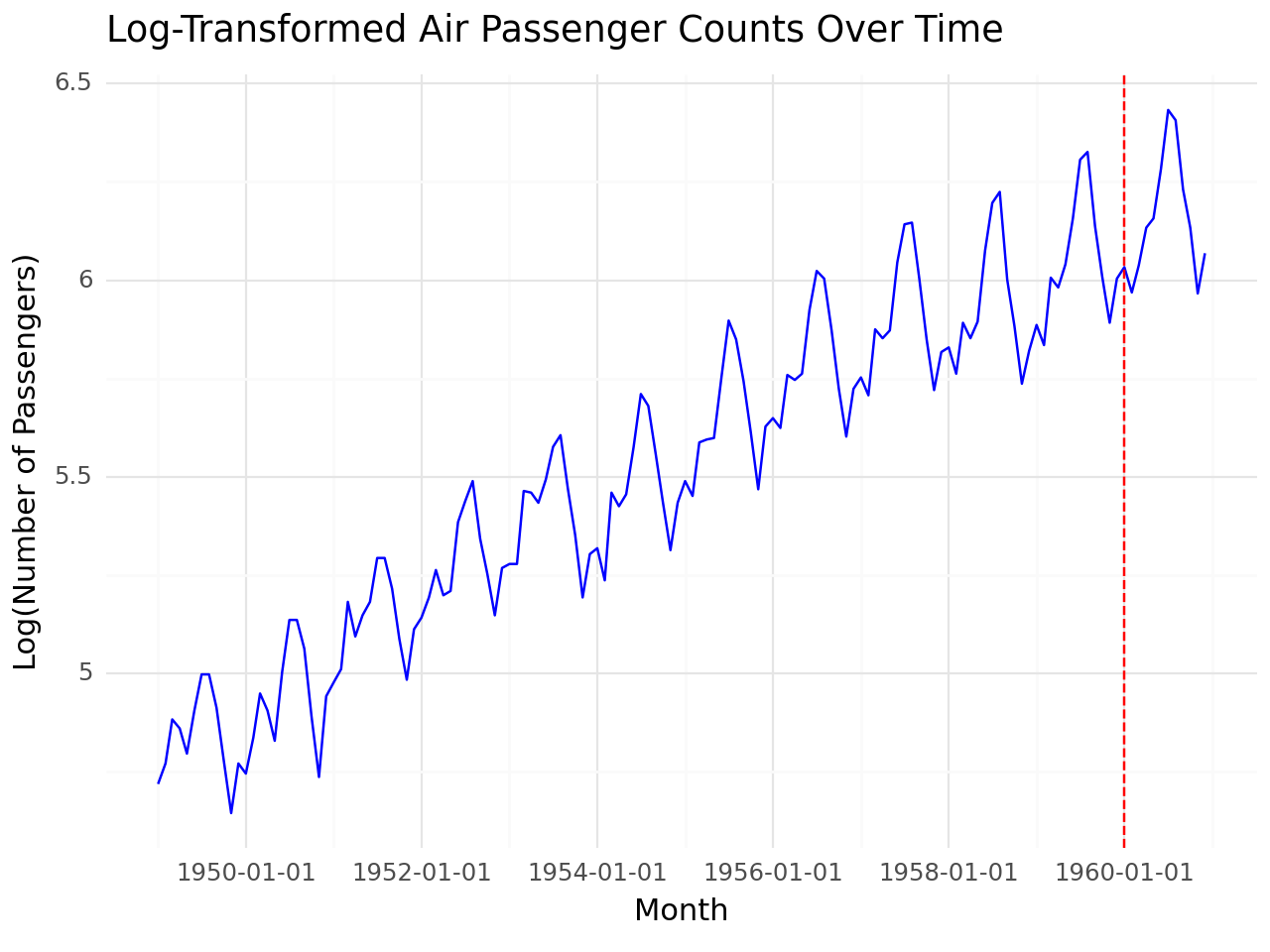

Set training data set and test dataset

training_data = airpassenger[airpassenger['Month'] < pd.to_datetime(split_date)]
test_data = airpassenger[airpassenger['Month'] >= pd.to_datetime(split_date)]

Plot ACF and PACF for training data

import matplotlib.pyplot as plt
from statsmodels.graphics.tsaplots import plot_acf, plot_pacf
plt.figure(figsize=(12, 6))
plt.subplot(1, 2, 1)
plot_acf(training_data['Log_Passengers'], lags=40, ax=plt.gca())
plt.title('ACF of Log-Transformed Training Data')

plt.subplot(1, 2, 2)
plot_pacf(training_data['Log_Passengers'], lags=40, ax=plt.gca(), method='ywm')
plt.title('PACF of Log-Transformed Training Data')

plt.tight_layout()
plt.show()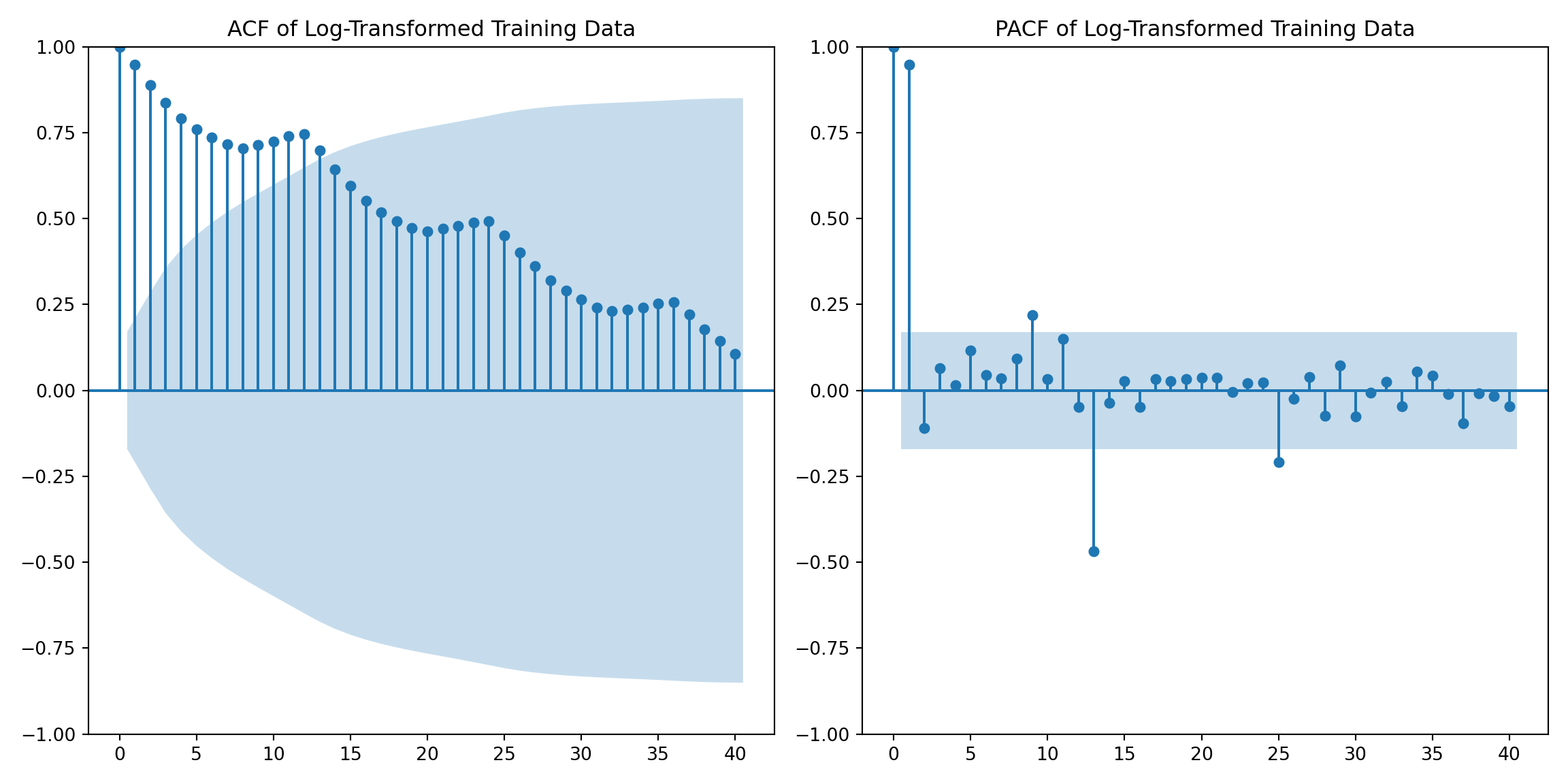

Apply First-Order Seasonal Difference and Obtain ACF and PACF

airpassenger['LogSeasonal_Diff'] = airpassenger['Log_Passengers'] - airpassenger['Log_Passengers'].shift(12)
airpassenger.head(14)

	Month	#Passengers	Log_Passengers	LogSeasonal_Diff
0	1949-01-01	112	4.718499	NaN
1	1949-02-01	118	4.770685	NaN
2	1949-03-01	132	4.882802	NaN
3	1949-04-01	129	4.859812	NaN
4	1949-05-01	121	4.795791	NaN
5	1949-06-01	135	4.905275	NaN
6	1949-07-01	148	4.997212	NaN
7	1949-08-01	148	4.997212	NaN
8	1949-09-01	136	4.912655	NaN
9	1949-10-01	119	4.779123	NaN
10	1949-11-01	104	4.644391	NaN
11	1949-12-01	118	4.770685	NaN
12	1950-01-01	115	4.744932	0.026433
13	1950-02-01	126	4.836282	0.065597

airpassenger.tail(12)

	Month	#Passengers	Log_Passengers	LogSeasonal_Diff
132	1960-01-01	417	6.033086	0.146982
133	1960-02-01	391	5.968708	0.133897
134	1960-03-01	419	6.037871	0.031518
135	1960-04-01	461	6.133398	0.151984
136	1960-05-01	472	6.156979	0.116724
137	1960-06-01	535	6.282267	0.125288
138	1960-07-01	622	6.432940	0.126665
139	1960-08-01	606	6.406880	0.080731
140	1960-09-01	508	6.230481	0.092754
141	1960-10-01	461	6.133398	0.124585
142	1960-11-01	390	5.966147	0.074503
143	1960-12-01	432	6.068426	0.064539

Remove rows with NaN values from the airpassenger DataFrame

airpassenger.dropna(inplace=True)

# Display the cleaned DataFrame
print(airpassenger)

         Month  #Passengers  Log_Passengers  LogSeasonal_Diff
12  1950-01-01          115        4.744932          0.026433
13  1950-02-01          126        4.836282          0.065597
14  1950-03-01          141        4.948760          0.065958
15  1950-04-01          135        4.905275          0.045462
16  1950-05-01          125        4.828314          0.032523
..         ...          ...             ...               ...
139 1960-08-01          606        6.406880          0.080731
140 1960-09-01          508        6.230481          0.092754
141 1960-10-01          461        6.133398          0.124585
142 1960-11-01          390        5.966147          0.074503
143 1960-12-01          432        6.068426          0.064539

[132 rows x 4 columns]

Plot ACF and PACF of the log-seasonally differenced series

fig, axes = plt.subplots(1, 2, figsize=(16, 6))

# ACF plot
plot_acf(airpassenger['LogSeasonal_Diff'], ax=axes[0], lags=40)
axes[0].set_title('ACF of Log-Seasonally Differenced Series')

# PACF plot
plot_pacf(airpassenger['LogSeasonal_Diff'], ax=axes[1], lags=40)
axes[1].set_title('PACF of Log-Seasonally Differenced Series')

plt.tight_layout()
plt.show()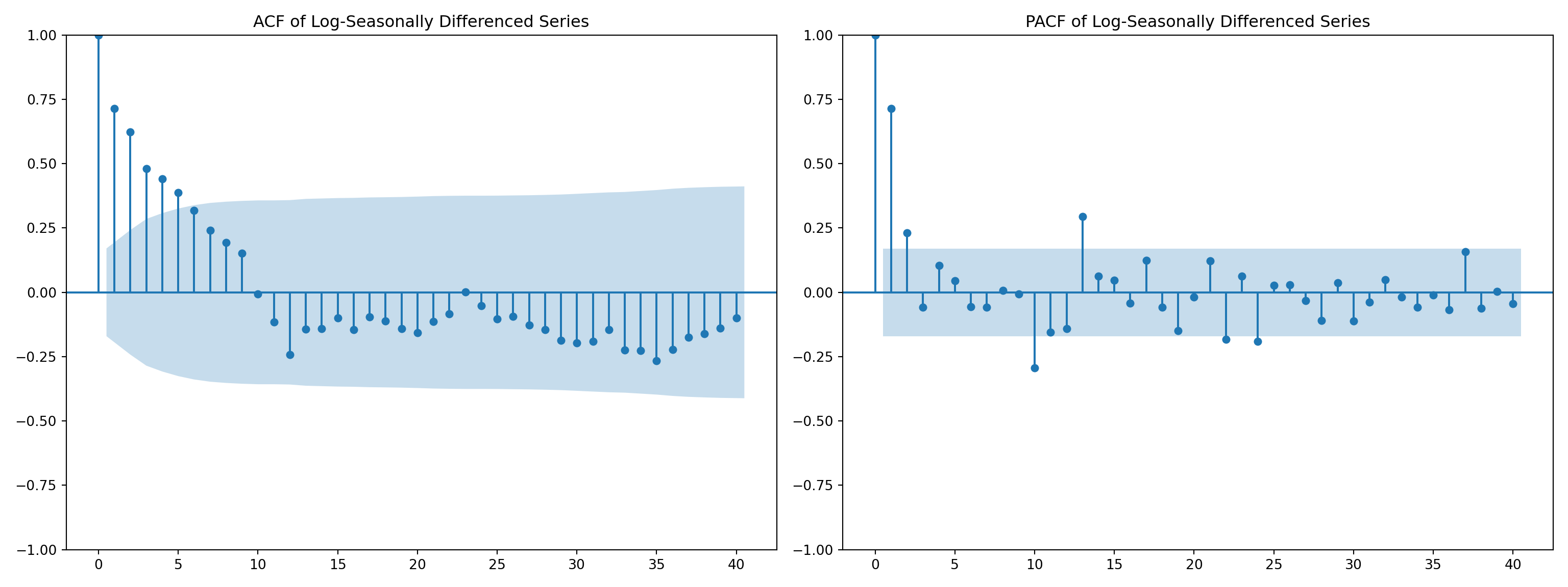

Apply First-Order Differencing

airpassenger['LogSeasonal_Diff.NonSeaDiff'] = airpassenger['LogSeasonal_Diff'] - airpassenger['LogSeasonal_Diff'].shift(1)
airpassenger.head(14)
airpassenger.dropna(inplace=True)

fig, axes = plt.subplots(1, 2, figsize=(16, 6))

# ACF plot
plot_acf(airpassenger['LogSeasonal_Diff.NonSeaDiff'], ax=axes[0], lags=40)
axes[0].set_title('ACF of Log-Seasonally Differenced and Non Seasonally Differenced Series')

# PACF plot
plot_pacf(airpassenger['LogSeasonal_Diff.NonSeaDiff'], ax=axes[1], lags=40)
axes[1].set_title('PACF of Log-Seasonally Differenced and Non-Seasonally DIfferenced Series')

plt.tight_layout()
plt.show()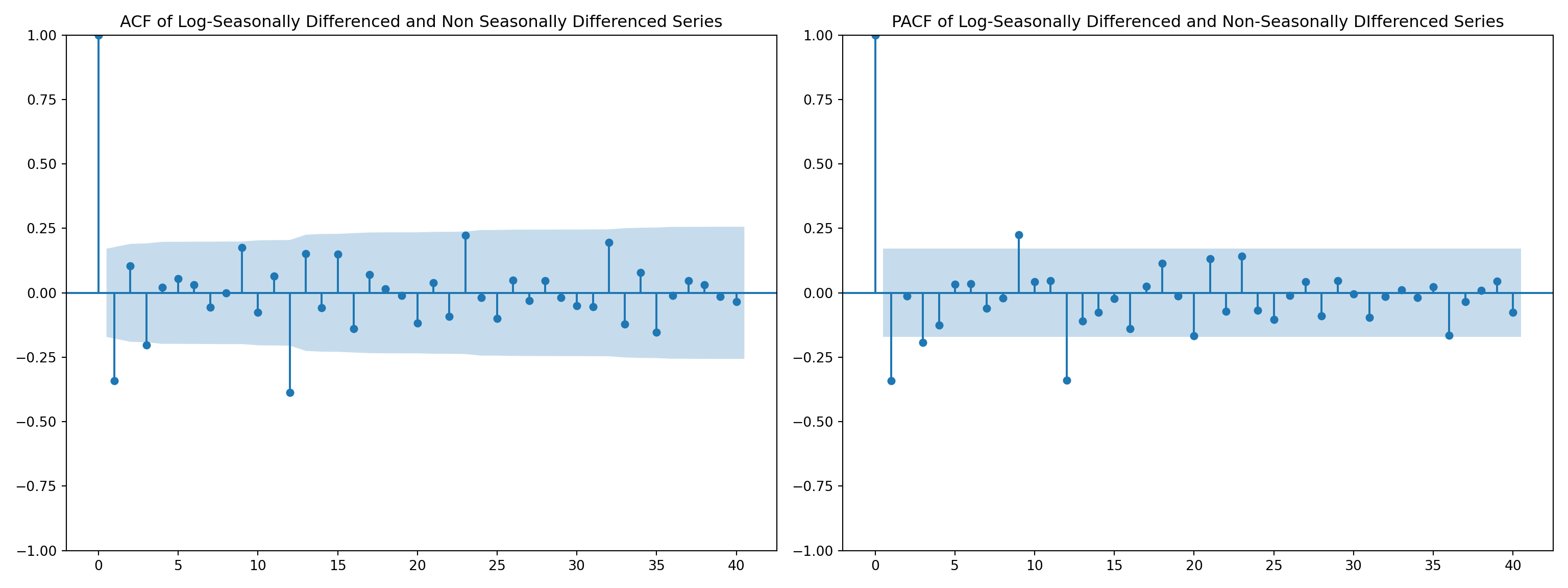

Fit ARIMA(0,1,1)(0,1,1)[12] model

from statsmodels.tsa.arima.model import ARIMA
model = ARIMA(airpassenger['Log_Passengers'], order=(0, 1, 1), seasonal_order=(0, 1, 1, 12))
fitted_model = model.fit()
forecast = fitted_model.forecast(steps=13)
forecast

C:\Users\DELL\AppData\Local\Programs\Python\Python312\Lib\site-packages\statsmodels\tsa\base\tsa_model.py:473: ValueWarning: An unsupported index was provided and will be ignored when e.g. forecasting.
C:\Users\DELL\AppData\Local\Programs\Python\Python312\Lib\site-packages\statsmodels\tsa\base\tsa_model.py:473: ValueWarning: An unsupported index was provided and will be ignored when e.g. forecasting.
C:\Users\DELL\AppData\Local\Programs\Python\Python312\Lib\site-packages\statsmodels\tsa\base\tsa_model.py:473: ValueWarning: An unsupported index was provided and will be ignored when e.g. forecasting.
C:\Users\DELL\AppData\Local\Programs\Python\Python312\Lib\site-packages\statsmodels\tsa\base\tsa_model.py:836: ValueWarning: No supported index is available. Prediction results will be given with an integer index beginning at `start`.
C:\Users\DELL\AppData\Local\Programs\Python\Python312\Lib\site-packages\statsmodels\tsa\base\tsa_model.py:836: FutureWarning: No supported index is available. In the next version, calling this method in a model without a supported index will result in an exception.

131    6.110396
132    6.053819
133    6.171650
134    6.199400
135    6.232725
136    6.368919
137    6.507530
138    6.503117
139    6.324834
140    6.209196
141    6.063624
142    6.168173
143    6.206753
Name: predicted_mean, dtype: float64

Residual Analysis

import seaborn as sns
# Compute residuals
train_forecast = fitted_model.fittedvalues
residuals = airpassenger['Log_Passengers'] - train_forecast

# Plot residuals
plt.figure(figsize=(10, 6))
plt.plot(airpassenger['Month'], residuals, label='Residuals', color='purple')
plt.axhline(0, color='black', linewidth=1)
plt.title('Residuals from ARIMA Model')
plt.xlabel('Month')
plt.ylabel('Residuals')
plt.legend()
plt.grid(True)
plt.show()

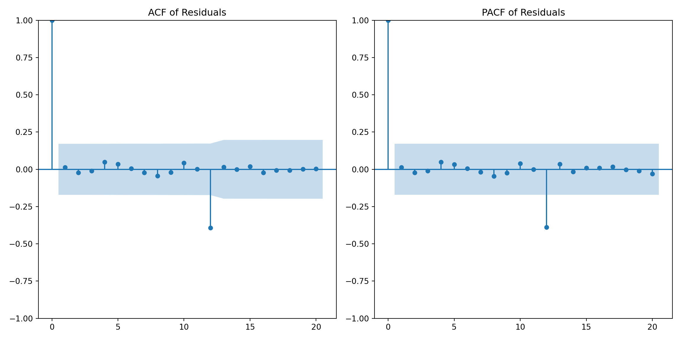
# Plot the ACF and PACF of residuals to check for autocorrelation
plt.figure(figsize=(12, 6))

plt.subplot(1, 2, 1)
plot_acf(residuals, lags=20, ax=plt.gca())
plt.title('ACF of Residuals')

plt.subplot(1, 2, 2)
plot_pacf(residuals, lags=20, ax=plt.gca())
plt.title('PACF of Residuals')

plt.tight_layout()
plt.show()

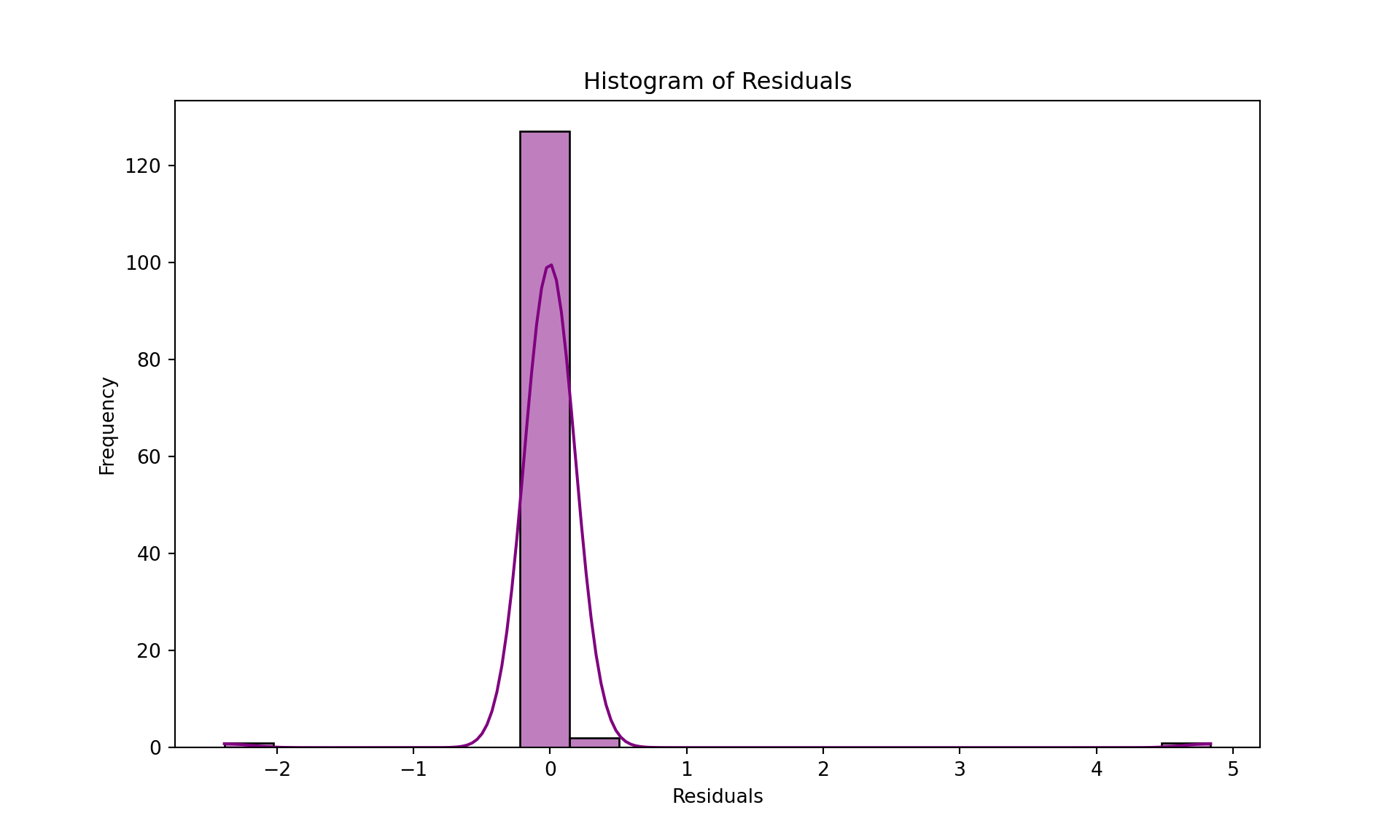
# Histogram of residuals to check for normality
plt.figure(figsize=(10, 6))
sns.histplot(residuals, kde=True, color='purple', bins=20)
plt.title('Histogram of Residuals')
plt.xlabel('Residuals')
plt.ylabel('Frequency')
plt.show()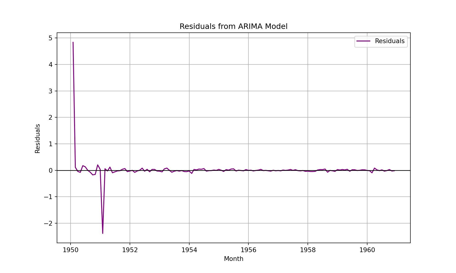

Back-transform forecasted log values to original scale

forecast_original = np.exp(forecast)
test_data['forecast_log'] = forecast
test_data['forecast_passengers'] = forecast_original
test_data

C:\Users\DELL\AppData\Local\Temp\ipykernel_9236\3410330437.py:2: SettingWithCopyWarning: 
A value is trying to be set on a copy of a slice from a DataFrame.
Try using .loc[row_indexer,col_indexer] = value instead

See the caveats in the documentation: https://pandas.pydata.org/pandas-docs/stable/user_guide/indexing.html#returning-a-view-versus-a-copy
C:\Users\DELL\AppData\Local\Temp\ipykernel_9236\3410330437.py:3: SettingWithCopyWarning: 
A value is trying to be set on a copy of a slice from a DataFrame.
Try using .loc[row_indexer,col_indexer] = value instead

See the caveats in the documentation: https://pandas.pydata.org/pandas-docs/stable/user_guide/indexing.html#returning-a-view-versus-a-copy

	Month	#Passengers	Log_Passengers	forecast_log	forecast_passengers
132	1960-01-01	417	6.033086	6.053819	425.735873
133	1960-02-01	391	5.968708	6.171650	478.975744
134	1960-03-01	419	6.037871	6.199400	492.453690
135	1960-04-01	461	6.133398	6.232725	509.141110
136	1960-05-01	472	6.156979	6.368919	583.426973
137	1960-06-01	535	6.282267	6.507530	670.168960
138	1960-07-01	622	6.432940	6.503117	667.218211
139	1960-08-01	606	6.406880	6.324834	558.265074
140	1960-09-01	508	6.230481	6.209196	497.301356
141	1960-10-01	461	6.133398	6.063624	429.930518
142	1960-11-01	390	5.966147	6.168173	477.313188
143	1960-12-01	432	6.068426	6.206753	496.087694

Compute MSE

from sklearn.metrics import mean_squared_error
mse = mean_squared_error(test_data['#Passengers'], test_data['forecast_passengers'])

print(f'Mean Squared Error (MSE): {mse}')

Mean Squared Error (MSE): 5279.13204916217

Loading packages

Read data

Visualise data

Training set vs Test set

Apply log transformation

Set training data set and test dataset

Plot ACF and PACF for training data

Apply First-Order Seasonal Difference and Obtain ACF and PACF

Remove rows with NaN values from the airpassenger DataFrame

Plot ACF and PACF of the log-seasonally differenced series

Apply First-Order Differencing

Fit ARIMA(0,1,1)(0,1,1)[12] model

Residual Analysis

Back-transform forecasted log values to original scale

Compute MSE

Your turn: Write R codes to identify the suitable SARIMA model for AirPassengers dataset.