import pandas as pd
import plotnine as p9
from plotnine import *
from plotnine.data import *
import numpy as npTime Series Forecasting with Python: Method 2
Loading packages
Modelling steps
Plot the data.
If necessary, transform the data (using a Box-Cox transformation) to stabilise the variance.
3. If the data are non-stationary, take first differences of the data until the data are stationary.
4. Examine the ACF/PACF to identify a suitable model.
5. Try your chosen model(s), and use the AICc to search for a better model.
Check the residuals from your chosen model by plotting the ACF of the residuals, and doing a portmanteau test of the residuals. If they do not look like white noise, try a modified model.
Once the residuals look like white noise, calculate forecasts.
Modelling steps: AutoARIMA
Plot the data.
If necessary, transform the data (using a Box-Cox transformation) to stabilise the variance.
Use AutoARIMA to select a model.
Check the residuals from your chosen model by plotting the ACF of the residuals, and doing a portmanteau test of the residuals. If they do not look like white noise, try a modified model.
Once the residuals look like white noise, calculate forecasts.
Modeling with Python
from sktime import *
from sktime.datasets import load_airline
from sktime.utils.plotting import plot_series
y = load_airline()
plot_series(y)
(<Figure size 1536x384 with 1 Axes>,
<Axes: ylabel='Number of airline passengers'>)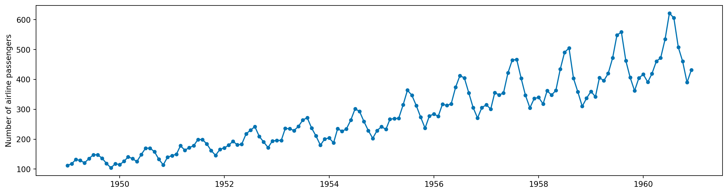
Your turn
Take other important visualizations
Define forecast horizon
import numpy as np
import pandas as pd
from sktime.forecasting.base import ForecastingHorizon
fh = ForecastingHorizon(
    pd.PeriodIndex(pd.date_range("1960-01", periods=12, freq="M")), is_relative=False
)
fh
ForecastingHorizon(['1960-01', '1960-02', '1960-03', '1960-04', '1960-05', '1960-06',
'1960-07', '1960-08', '1960-09', '1960-10', '1960-11', '1960-12'],
dtype='period[M]', is_relative=False)Split data into training and test
from sktime.forecasting.model_selection import temporal_train_test_split
y_train, y_test = temporal_train_test_split(y, fh=fh)
Define forecaster with sktime
from sktime.forecasting.statsforecast import StatsForecastAutoARIMA
import numpy as np
forecaster = StatsForecastAutoARIMA(
    sp=12,  max_p=2, max_q=2
)
y_train.naturallog = np.log(y_train)
forecaster.fit(y_train.naturallog)
StatsForecastAutoARIMA(max_p=2, max_q=2, sp=12)Please rerun this cell to show the HTML repr or trust the notebook.
StatsForecastAutoARIMA(max_p=2, max_q=2, sp=12)
sp: Number of observations per unit of time.
Help: https://www.sktime.org/en/stable/api_reference/auto_generated/sktime.forecasting.statsforecast.StatsForecastAutoARIMA.html
Your turn
Preferm residual analysis
Obtain predictions for the training period
y_pred = forecaster.predict(fh)
y_pred
1960-01 6.038882
1960-02 5.989590
1960-03 6.146032
1960-04 6.119674
1960-05 6.159455
1960-06 6.304701
1960-07 6.432675
1960-08 6.444805
1960-09 6.266803
1960-10 6.136178
1960-11 6.007715
1960-12 6.114486
Freq: M, Name: Number of airline passengers, dtype: float64Model parameter estimates
Write a code to obtain model parameter estimates.
What is happening under the hood of AutoARIMA?
Step 1: Select the number of differences d and D via unit root tests and strength of seasonality measure.
Step 2: Try four possible models to start with:
\(ARIMA(2, d, 2)\) if \(m = 1\) and \(ARIMA(2, d, 2)(1, D, 1)_m\) if \(m > 1\).
\(ARIMA(0, d, 0)\) if \(m = 1\) and \(ARIMA(0, d, 0)(0, D, 0)_m\) if \(m > 1\).
\(ARIMA(1, d, 0)\) if \(m = 1\) and \(ARIMA(1, d, 0)(1, D, 0)_m\) if \(m > 1\).
\(ARIMA(0, d, 1)\) if \(m = 1\) and \(ARIMA(0, d, 1)(0, D, 1)_m\) if \(m > 1\).
Step 3: Select the model with the smallest AICc from step 2. This becomes the current model.
Step 4: Consider up to 13 variations on the current model:
Vary one of \(p, q, P\) and \(Q\) from the current model by \(\pm 1\).
\(p, q\) both vary from the current model by \(\pm 1\).
\(P, Q\) both vary from the current model by \(\pm 1\).
Include or exclude the constant term from the current model. Repeat step 4 until no lower AICc can be found.