Spatial Visualization with Python

Loading packages

import geopandas as gpd
import folium

Load and inspect meuse data

meuse = gpd.read_file("meuse.shp")  # Adjust the file path as needed

# Inspect the first few rows of the data
print(meuse.head())

   cadmium  copper   lead    zinc   elev      dist    om ffreq soil lime  \
0     11.7    85.0  299.0  1022.0  7.909  0.001358  13.6     1    1    1   
1      8.6    81.0  277.0  1141.0  6.983  0.012224  14.0     1    1    1   
2      6.5    68.0  199.0   640.0  7.800  0.103029  13.0     1    1    1   
3      2.6    81.0  116.0   257.0  7.655  0.190094   8.0     1    2    0   
4      2.8    48.0  117.0   269.0  7.480  0.277090   8.7     1    2    0   

  landuse  dist_m                       geometry  
0      Ah    50.0  POINT (181072.000 333611.000)  
1      Ah    30.0  POINT (181025.000 333558.000)  
2      Ah   150.0  POINT (181165.000 333537.000)  
3      Ga   270.0  POINT (181298.000 333484.000)  
4      Ah   380.0  POINT (181307.000 333330.000)  

Visualise the data

import matplotlib.pyplot as plt

# Plot the meuse dataset (points in this case)
meuse.plot(marker='o', color='blue', markersize=5)

# Show the plot
plt.title('Meuse Spatial Data Visualization')
plt.xlabel('Longitude')
plt.ylabel('Latitude')
plt.show()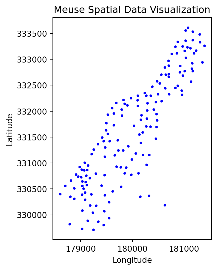

Customize plot

meuse.plot(column='zinc', cmap='viridis', legend=True, markersize=5)

# Show the plot
plt.title('Zinc Concentration in Meuse Data')
plt.xlabel('Longitude')
plt.ylabel('Latitude')
plt.show()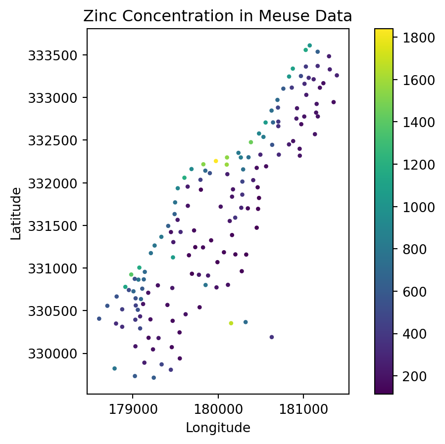

# Ensure the GeoDataFrame has the correct CRS and reproject to WGS84 for folium
gdf = meuse.to_crs(epsg=4326)

# Create a folium map centered on the data
map_center = [gdf.geometry.y.mean(), gdf.geometry.x.mean()]
m = folium.Map(location=map_center, zoom_start=12)

# Add points to the map with a popup for one of the attributes
for _, row in gdf.iterrows():
    folium.CircleMarker(
        location=[row.geometry.y, row.geometry.x],
        radius=5,
        color='blue',
        fill=True,
        fill_opacity=0.6,
        popup=f"Zinc: {row['zinc']}"  # Replace 'zinc' with a column from your shapefile
    ).add_to(m)

# Save or display the map
m.save("meuse_map.html")
m

Make this Notebook Trusted to load map: File -> Trust Notebook