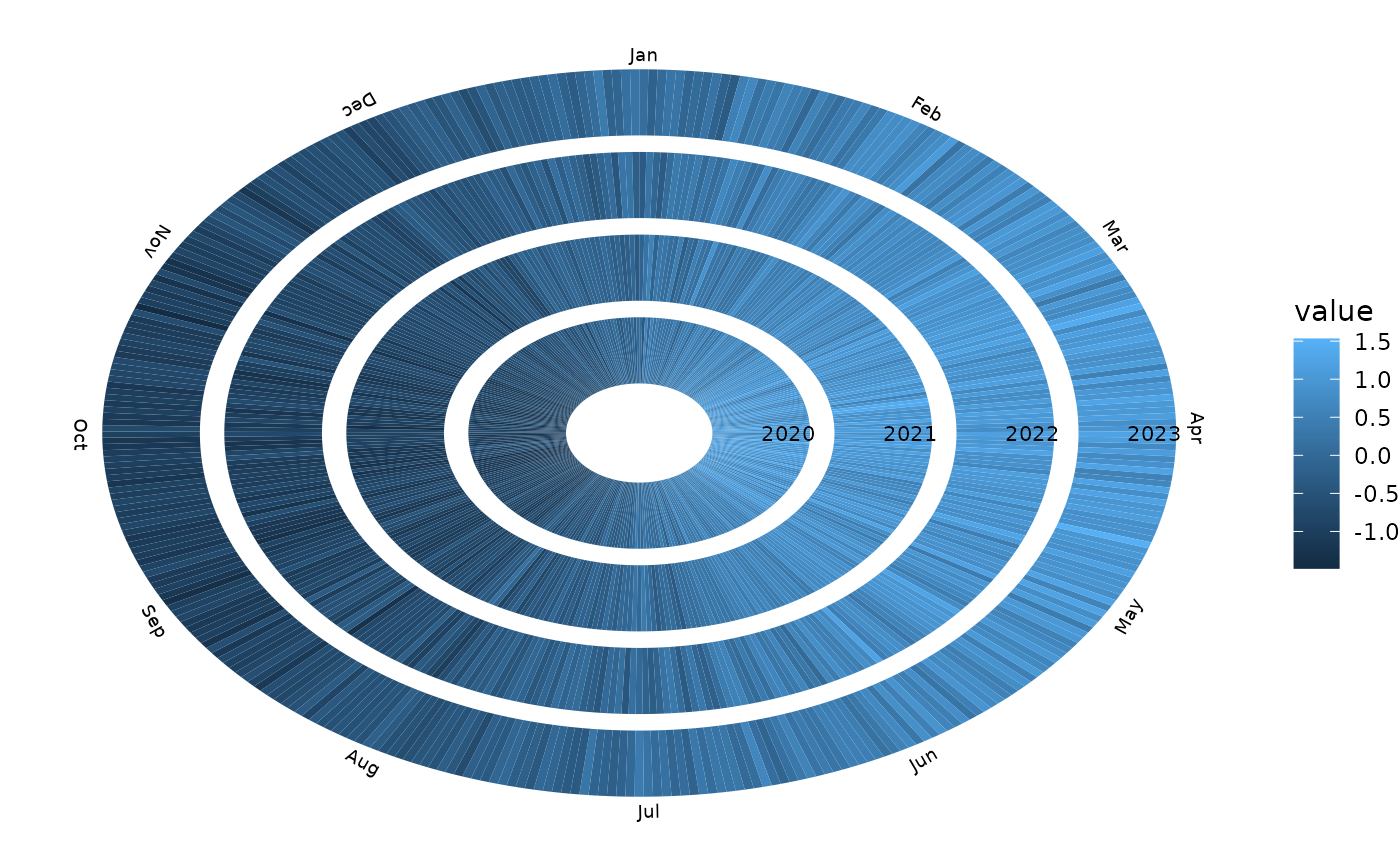
Create a spiral time-series plot using a fixed 365-day calendar.
Usage
geom_tsspiral(
  mapping = NULL,
  data = NULL,
  stat = StatTSSpiral,
  position = "identity",
  na.rm = FALSE,
  ring_spacing = 1,
  ...
)
Arguments
- mapping
Set of aesthetic mappings created by
ggplot2::aes().- data
A data frame, tibble, or tsibble containing the time-series data.
- stat
Statistical transformation used by the layer. Defaults to
StatTSSpiral.- position
Position adjustment. Defaults to
"identity".- na.rm
Logical. Should missing values be removed silently?
- ring_spacing
Numeric value controlling the distance between yearly rings.
- ...
Other arguments passed to
ggplot2::layer().
Details
geom_tsspiral() displays each year of a time series as a radial
ring. The angular position represents the day of the year. The
spiral always contains 365 angular divisions.
The spiral starts at 12 o'clock on January 1 and proceeds clockwise through the year.
The input frequency is detected automatically. Daily observations are used directly. Weekly, monthly, quarterly, and annual observations are expanded to daily observations before plotting.
Calendar labels are displayed only around the outermost ring:
daily data: month names,
monthly data: month names,
quarterly data: quarter names,
weekly data: week numbers,
annual data: month names.
The spiral uses a fixed 365-day calendar. January 1 starts at 12 o'clock and the calendar proceeds clockwise.
For day d, the angular position is
$$ \theta_d = \frac{\pi}{2} - \frac{2\pi(d-1)}{365}. $$
Consequently, January 1 is positioned at 12 o'clock and later days move clockwise around the spiral.
Leap years do not create a 366th angular division. February 29 is mapped to the February 28 position and the days after February 29 are shifted by one day.
Monthly, quarterly, weekly, and annual observations are expanded to their corresponding daily intervals. Consequently, a monthly observation fills the complete angular region corresponding to that month rather than appearing as a thin radial slice.
Examples
library(ggplot2)
#' # daily data
dat <- data.frame(
  date = seq.Date(
    as.Date("2020-01-01"),
    as.Date("2023-12-31"),
    by = "day"
  )
)
dat$value <- sin(
  2 * pi * as.numeric(format(dat$date, "%j")) / 365
) + rnorm(nrow(dat), sd = 0.2)

ggplot(
  dat,
  aes(
    x = date,
    y = value,
    fill = value
  )
) +
  geom_tsspiral(ring_spacing = 2) +
  theme_void()