3 Decision Trees

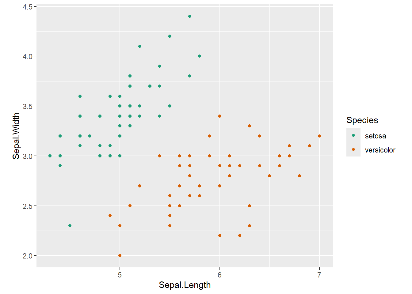
3.1 Motivational Example Dataset

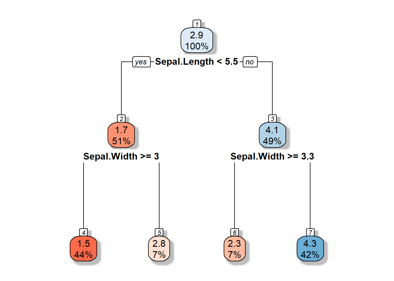
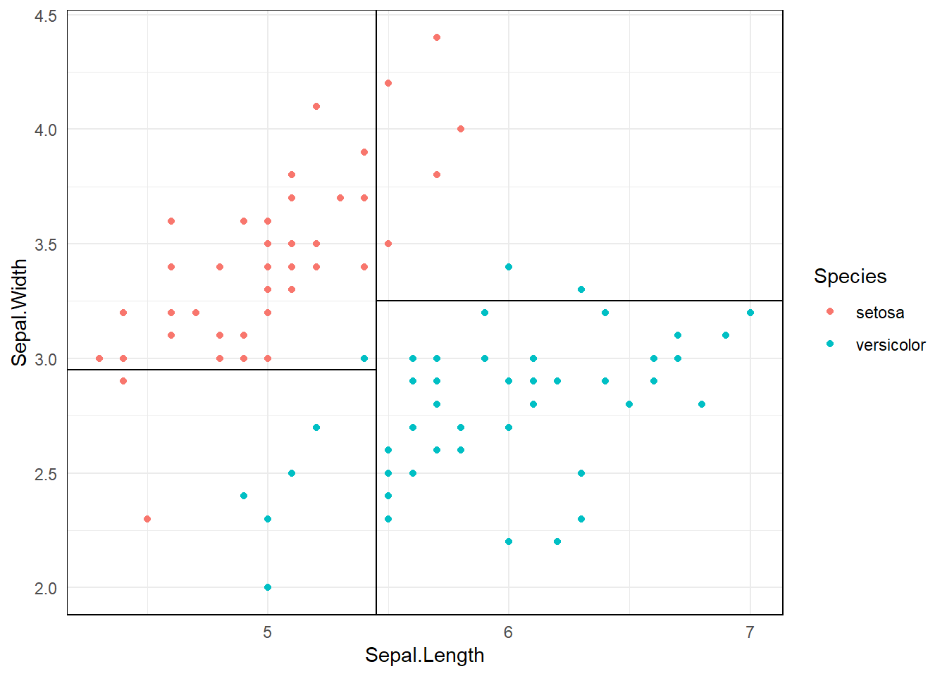
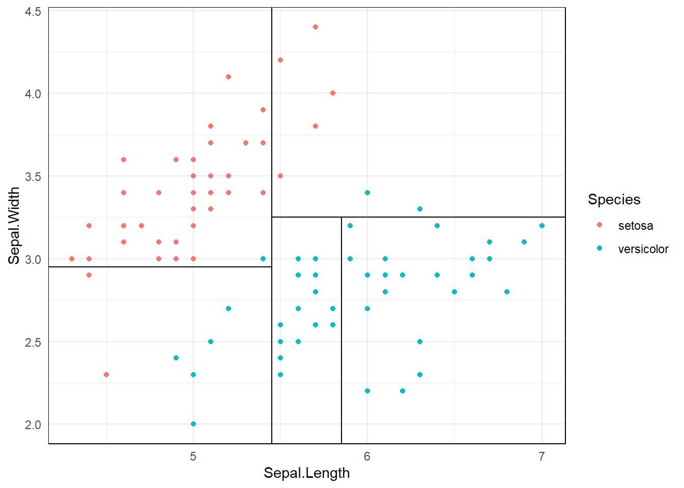
Features: Sepal Length, Sepal Width

Outcome: Species: setosa/versicolor

3.1.1 Predictor space

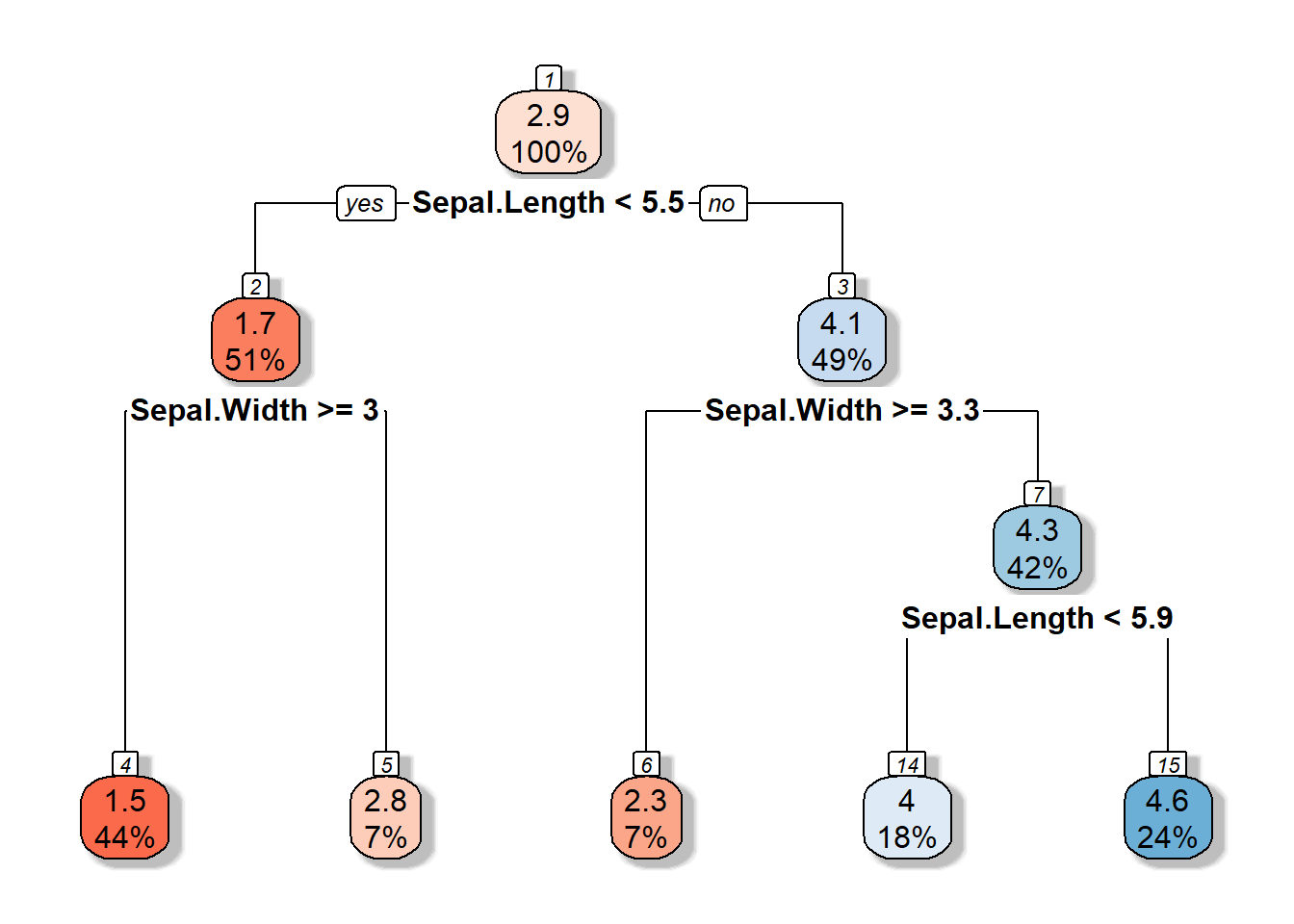
3.1.2 Decision Tree

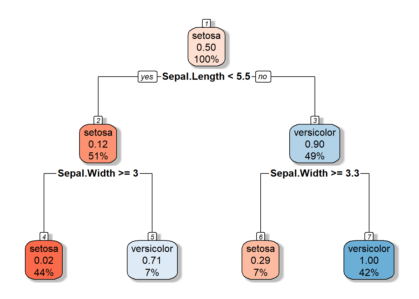
3.1.3 Partition space

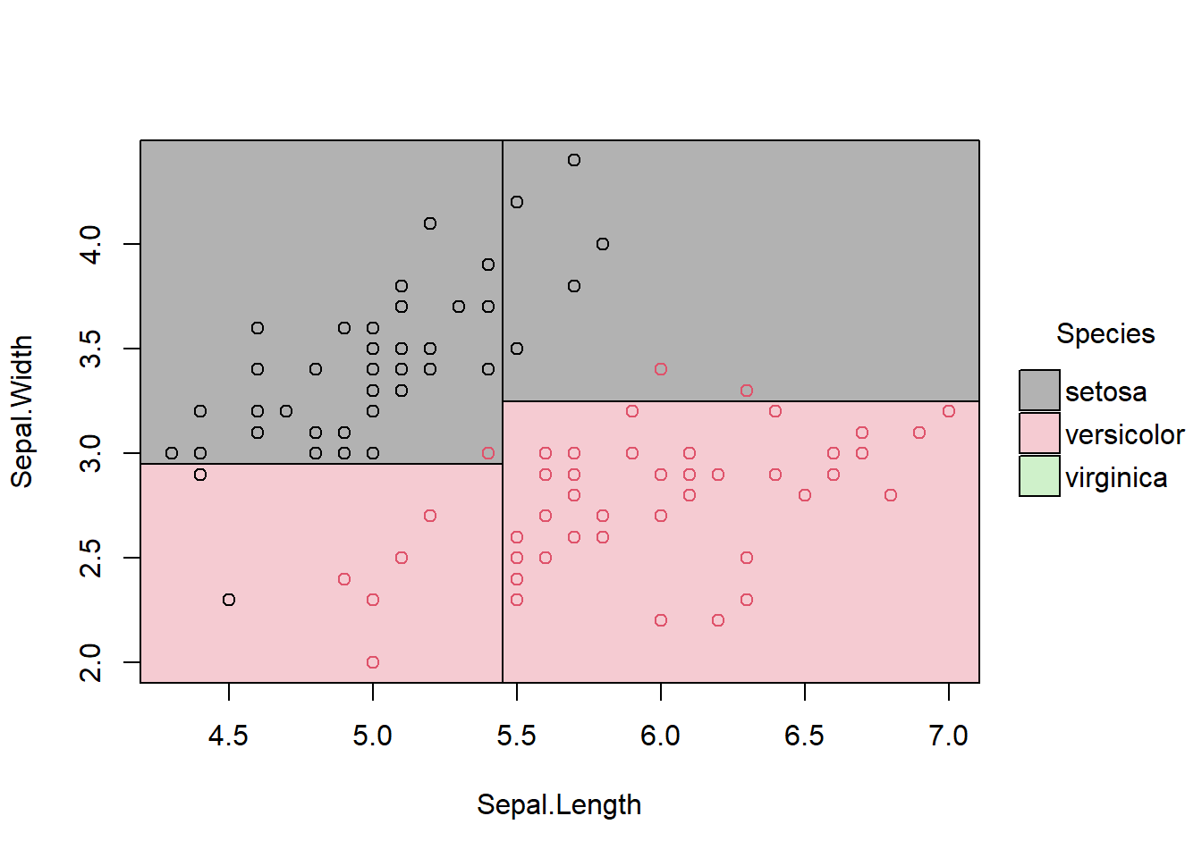
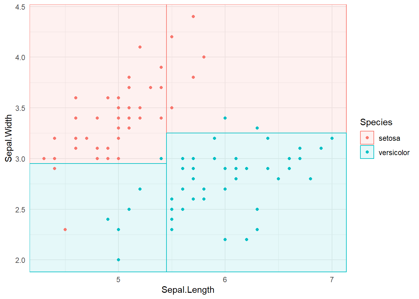
\(R1 = \{X|Sepal.Width >=3, Sepal.Length <5.5 \}\)

3.2 Parts of a decision tree

Root node
Decision node
Terminal node/ Leaf node (gives outputs/class assignments)
Subtree

3.3 Introduction

What happens in the model training phase?

Stratify or segment the predictor space into a number of non-overlapping regions.
Set of splitting rules are used to segment the predictor space.
Decision tree consists of a series of splitting rules.

How to make predictions?

Mean or mode response value for the training observations in the region which the observation we want to predict belong to.
We make the same prediction, for the training observations in the \(j^{th}\) region \(R_j\).

3.4 Decision Trees: Regression - Finding the best split and best splitting variable

The goal is to find \(R_1, R_2, R_3...R_J\), \(J\) distinct and non-overlapping regions that minimize the RSS given by

\[\sum_{j=1}^{J}\sum_{i \in R_j}(y_i - \hat{y}_{R_j})^2.\] \(\hat{y}_{R_j}\) - mean response for the training observations within the \(j^{th}\) region.

In theory, to build the best possible decision tree, we could try every possible way of splitting the data at every step and choose the one that gives the best results. However, this is computationally infeasible, especially when the dataset is large or when there are many predictor variables — the number of possible splits grows exponentially.

Therefore, instead of trying all possible combinations at once, we use a recursive partitioning approach. This means:

Start with the entire dataset as one group (the root node).

Find the single best split — the one that most effectively separates the data based on the target variable.

Divide the data into two or more subgroups (child nodes) based on that split.

Repeat the process (recursively) within each subgroup: again find the best split, divide the data, and continue until a stopping rule is met (for example, minimum node size or maximum tree depth).

This recursive process allows the algorithm to build the tree step by step, finding locally optimal splits that approximate the best possible tree without having to evaluate every possible combination.

3.5 Recursive Partitioning for Regression Trees

A regression tree predicts a continuous outcome (for example, house price, temperature, or pH level). The goal is to split the data into smaller and smaller groups (nodes) that are as homogeneous as possible with respect to the response variable.

In-class notation

3.6 Recursive Partitioning for Regression Trees

A regression tree is used when the response variable is continuous (e.g., house price, temperature, or pH level).

The goal is to split the data into smaller and smaller groups (nodes) that are as homogeneous as possible with respect to the response.

3.6.1 Step 1: Start with All Predictors

At the beginning, the algorithm considers all predictor variables:

\[X_1, X_2, X_3, \dots, X_p\]

For each predictor, it looks for the best split point that divides the data into two groups such that the prediction error (usually the sum of squared errors, SSE) is minimized.

3.6.2 Step 2: Consider All Possible Values

3.6.2.1 Continuous predictors

If a predictor \(X_j\) is continuous,
then “all possible values” refers to all unique values (or midpoints between consecutive sorted values) that can be used to split the data.

Example:

Observation	\(X_j\)
1	2
2	3
3	5
4	7

Possible split points (midpoints): - \(X_j < 2.5\) - \(X_j < 4\) - \(X_j < 6\)

Each of these potential splits is tested to see how well it reduces the SSE of the response variable.

3.6.2.2 Categorical predictors

If \(X_j\) is categorical,
“all possible values” means all possible groupings (subsets) of the categories.

Example:
If the predictor Species = {A, B, C}, possible splits are:

{A} vs {B, C}
{B} vs {A, C}
{C} vs {A, B}

Each grouping is evaluated based on how much it reduces the variability in the response.

3.6.3 Step 3: Choose the Best Split

For every predictor and every possible split value, compute:

\[ \text{SSE}_{\text{split}} = \text{SSE}_{\text{left node}} + \text{SSE}_{\text{right node}} \]

The split that minimizes this total SSE is chosen as the best split for that node.

3.6.4 Step 4: Recursive Partitioning

After splitting the data into two nodes, the same process is applied recursively within each node:

Consider all predictors again.
For each predictor, test all possible values.
Find the best split within that node.
Continue until a stopping rule is met (e.g., minimum node size or no significant improvement).

3.6.5 Summary

Concept	Explanation
All predictors	Every variable \(X_1, X_2, \dots, X_p\) is considered at each split.
All possible values	Every unique value (or midpoint between values) is tested as a potential split.
Recursive partitioning	The process of repeatedly splitting the data into smaller homogeneous groups until a stopping rule is met.

In summary:
Finding every possible combination of splits is computationally infeasible.
Recursive partitioning provides a practical, step-by-step method that finds locally optimal splits efficiently.

3.7 Depth of the decision tree

3.8 Pruning Regression Trees

Once a regression tree is grown, it often becomes too complex — it may fit the training data very well but perform poorly on new, unseen data.
This problem is known as overfitting.

Pruning is the process of reducing the size of a fully grown tree to improve its ability to generalize.

3.8.1 Why Prune?

A large tree captures noise as if it were structure.
It has low bias but high variance.
Pruning helps to find a balance between model complexity and prediction accuracy.

3.8.2 Types of Pruning

There are two main approaches:

3.8.2.1 (a) Pre-pruning (Early stopping)

Stop the tree growth before it becomes too large.

Common stopping rules:

Minimum number of observations in a node
Maximum tree depth
Minimum decrease in SSE required for a split

3.8.2.2 (b) Post-pruning (Cost Complexity Pruning)

Grow a large tree first, then prune it backward by removing branches that contribute little to predictive accuracy.

3.8.3 Cost Complexity Pruning (a.k.a. Weakest Link Pruning)

The idea is to penalize tree size using a complexity parameter (\(\lambda\)).

For any subtree ( T ):

\[ C(T) = \text{Error}(T) + \lambda L(T) \]

where:

(T): measure of fit (e.g., sum of squared errors)
\(L(T)\): number of leaf nodes in the tree (measure of complexity)
\(\lambda\): penalty factor controlling the trade-off between complexity and predictive power

3.8.4 Interpretation of Parameters

Parameter	Meaning
\(\lambda = 0\)	Fully grown decision tree (no penalty for complexity).
\(\lambda = \infty\)	Root node only (maximum penalty, no splits).
\(0 < \lambda < \infty\)	Balances predictive power and complexity.

3.8.5 Total Cost Components

\[ \text{Total Cost} = \text{Measure of Fit} + \text{Measure of Complexity} \]

Measure of Fit: Error (e.g., SSE)
Measure of Complexity: Number of leaf nodes \(L(T)\)

So, \[ C(T) = \text{Error}(T) + \lambda L(T) \]

This is sometimes written as:

\[ R_\lambda(T) = R(T) + \lambda |T| \]

Both expressions represent the same concept — a trade-off between model fit and simplicity.

3.9 Example R code for Pre-pruning and Post-pruning

# Load necessary packages
library(rpart)
library(rpart.plot)

# Use built-in dataset
data(mtcars)

# -----------------------------
# 🌱 1. Pre-pruning (Early stopping)
# -----------------------------
# Control parameters limit tree growth
prepruned_tree <- rpart(
  mpg ~ ., 
  data = mtcars,
  method = "anova",
  control = rpart.control(
    minsplit = 10,   # minimum observations required to attempt a split
    cp = 0.02,       # minimum improvement in SSE required for a split
    maxdepth = 3     # maximum depth of the tree
  )
)

# Visualize the pre-pruned tree
rpart.plot(prepruned_tree, main = "Pre-pruned Regression Tree")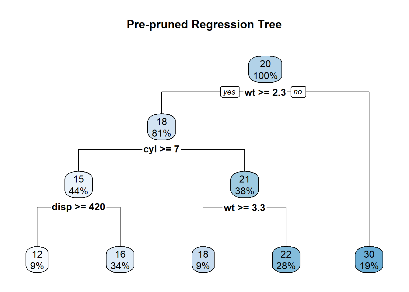

# Print summary
print(prepruned_tree)

n= 32 

node), split, n, deviance, yval
      * denotes terminal node

 1) root 32 1126.047000 20.09062  
   2) wt>=2.26 26  346.566500 17.78846  
     4) cyl>=7 14   85.200000 15.10000  
       8) disp>=420 3   12.326670 11.83333 *
       9) disp< 420 11   32.129090 15.99091 *
     5) cyl< 7 12   42.122500 20.92500  
      10) wt>=3.3275 3    1.086667 18.36667 *
      11) wt< 3.3275 9   14.855560 21.77778 *
   3) wt< 2.26 6   44.553330 30.06667 *

summary(prepruned_tree)

Call:
rpart(formula = mpg ~ ., data = mtcars, method = "anova", control = rpart.control(minsplit = 10, 
    cp = 0.02, maxdepth = 3))
  n= 32 

          CP nsplit rel error    xerror       xstd
1 0.65266121      0 1.0000000 1.0863063 0.26519210
2 0.19470235      1 0.3473388 0.6852332 0.16791734
3 0.03618342      2 0.1526364 0.3430358 0.10012133
4 0.02324972      3 0.1164530 0.2957831 0.07419667
5 0.02000000      4 0.0932033 0.2887422 0.07322052

Variable importance
  wt disp   hp drat  cyl qsec   vs 
  27   25   19   11    9    5    5 

Node number 1: 32 observations,    complexity param=0.6526612
  mean=20.09062, MSE=35.18897 
  left son=2 (26 obs) right son=3 (6 obs)
  Primary splits:
      wt   < 2.26   to the right, improve=0.6526612, (0 missing)
      cyl  < 5      to the right, improve=0.6431252, (0 missing)
      disp < 163.8  to the right, improve=0.6130502, (0 missing)
      hp   < 118    to the right, improve=0.6010712, (0 missing)
      vs   < 0.5    to the left,  improve=0.4409477, (0 missing)
  Surrogate splits:
      disp < 101.55 to the right, agree=0.969, adj=0.833, (0 split)
      hp   < 92     to the right, agree=0.938, adj=0.667, (0 split)
      drat < 4      to the left,  agree=0.906, adj=0.500, (0 split)
      cyl  < 5      to the right, agree=0.844, adj=0.167, (0 split)

Node number 2: 26 observations,    complexity param=0.1947024
  mean=17.78846, MSE=13.32948 
  left son=4 (14 obs) right son=5 (12 obs)
  Primary splits:
      cyl  < 7      to the right, improve=0.6326174, (0 missing)
      disp < 266.9  to the right, improve=0.6326174, (0 missing)
      hp   < 136.5  to the right, improve=0.5803554, (0 missing)
      wt   < 3.325  to the right, improve=0.5393370, (0 missing)
      qsec < 18.15  to the left,  improve=0.4210605, (0 missing)
  Surrogate splits:
      disp < 266.9  to the right, agree=1.000, adj=1.000, (0 split)
      hp   < 136.5  to the right, agree=0.962, adj=0.917, (0 split)
      wt   < 3.49   to the right, agree=0.885, adj=0.750, (0 split)
      qsec < 18.15  to the left,  agree=0.885, adj=0.750, (0 split)
      vs   < 0.5    to the left,  agree=0.885, adj=0.750, (0 split)

Node number 3: 6 observations
  mean=30.06667, MSE=7.425556 

Node number 4: 14 observations,    complexity param=0.03618342
  mean=15.1, MSE=6.085714 
  left son=8 (3 obs) right son=9 (11 obs)
  Primary splits:
      disp < 420    to the right, improve=0.4782188, (0 missing)
      wt   < 4.66   to the right, improve=0.4782188, (0 missing)
      hp   < 192.5  to the right, improve=0.4669349, (0 missing)
      carb < 3.5    to the right, improve=0.4669349, (0 missing)
      qsec < 17.71  to the right, improve=0.4306658, (0 missing)
  Surrogate splits:
      wt   < 4.66   to the right, agree=1.000, adj=1.000, (0 split)
      drat < 3.035  to the left,  agree=0.857, adj=0.333, (0 split)
      qsec < 17.41  to the right, agree=0.857, adj=0.333, (0 split)

Node number 5: 12 observations,    complexity param=0.02324972
  mean=20.925, MSE=3.510208 
  left son=10 (3 obs) right son=11 (9 obs)
  Primary splits:
      wt   < 3.3275 to the right, improve=0.6215272, (0 missing)
      cyl  < 5      to the right, improve=0.5573591, (0 missing)
      hp   < 96     to the right, improve=0.5507811, (0 missing)
      disp < 163.8  to the right, improve=0.4615111, (0 missing)
      carb < 3      to the right, improve=0.2857431, (0 missing)
  Surrogate splits:
      disp < 163.8  to the right, agree=0.917, adj=0.667, (0 split)
      hp   < 116.5  to the right, agree=0.833, adj=0.333, (0 split)

Node number 8: 3 observations
  mean=11.83333, MSE=4.108889 

Node number 9: 11 observations
  mean=15.99091, MSE=2.920826 

Node number 10: 3 observations
  mean=18.36667, MSE=0.3622222 

Node number 11: 9 observations
  mean=21.77778, MSE=1.650617

# -----------------------------
# 🌳 2. Post-pruning (Cost-complexity pruning)
# -----------------------------
# Step 1: Grow a large tree first
full_tree <- rpart(
  mpg ~ ., 
  data = mtcars,
  method = "anova",
  control = rpart.control(cp = 0.0001)  # allow the tree to grow large
)

# Step 2: Display complexity parameter (CP) table
printcp(full_tree)


Regression tree:
rpart(formula = mpg ~ ., data = mtcars, method = "anova", control = rpart.control(cp = 1e-04))

Variables actually used in tree construction:
[1] cyl hp 

Root node error: 1126/32 = 35.189

n= 32 

        CP nsplit rel error  xerror    xstd
1 0.643125      0   1.00000 1.02606 0.24552
2 0.097484      1   0.35687 0.64743 0.16940
3 0.000100      2   0.25939 0.53811 0.12137

# Step 3: Plot cross-validation results
plotcp(full_tree, main = "Cost-Complexity Pruning Plot")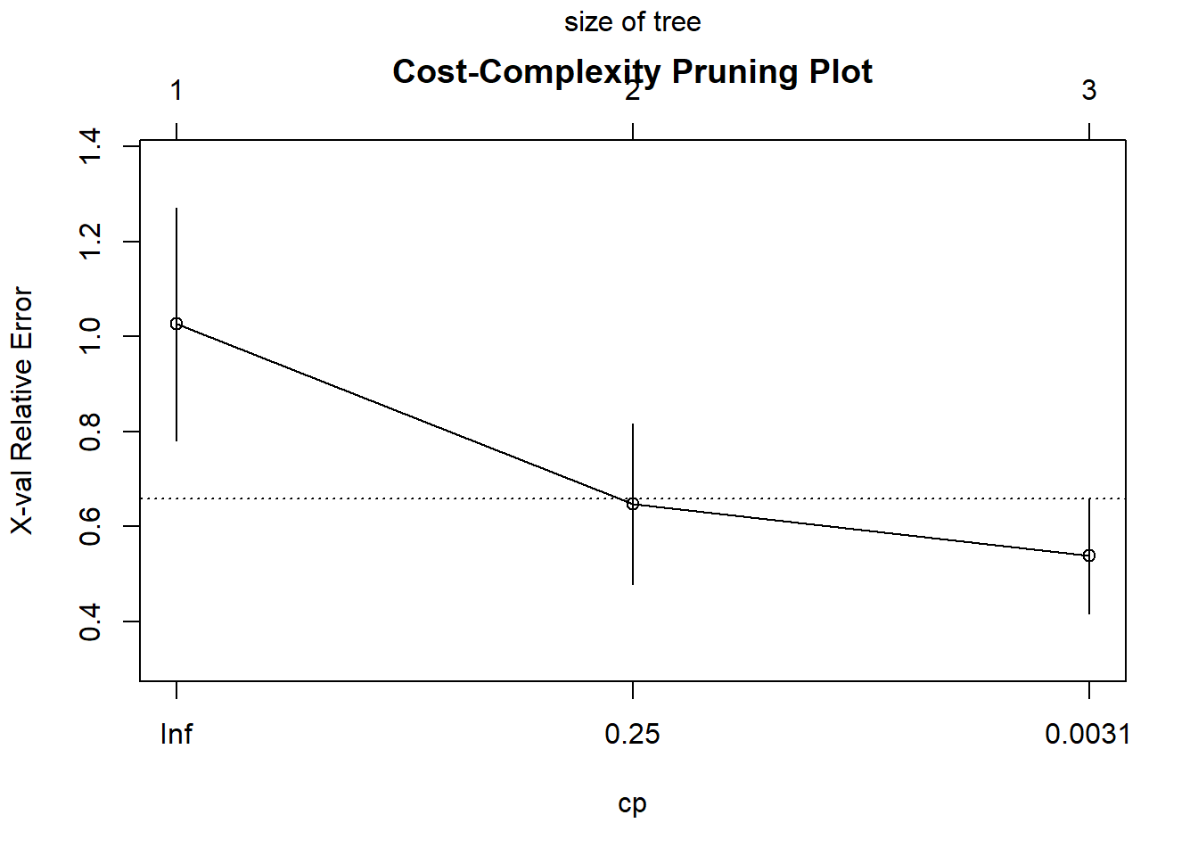

# Step 4: Select the cp value that minimizes cross-validation error
optimal_cp <- full_tree$cptable[which.min(full_tree$cptable[,"xerror"]), "CP"]

# Step 5: Prune the tree at the optimal cp value
pruned_tree <- prune(full_tree, cp = optimal_cp)

# Step 6: Visualize the pruned tree
rpart.plot(pruned_tree, main = "Post-pruned Regression Tree")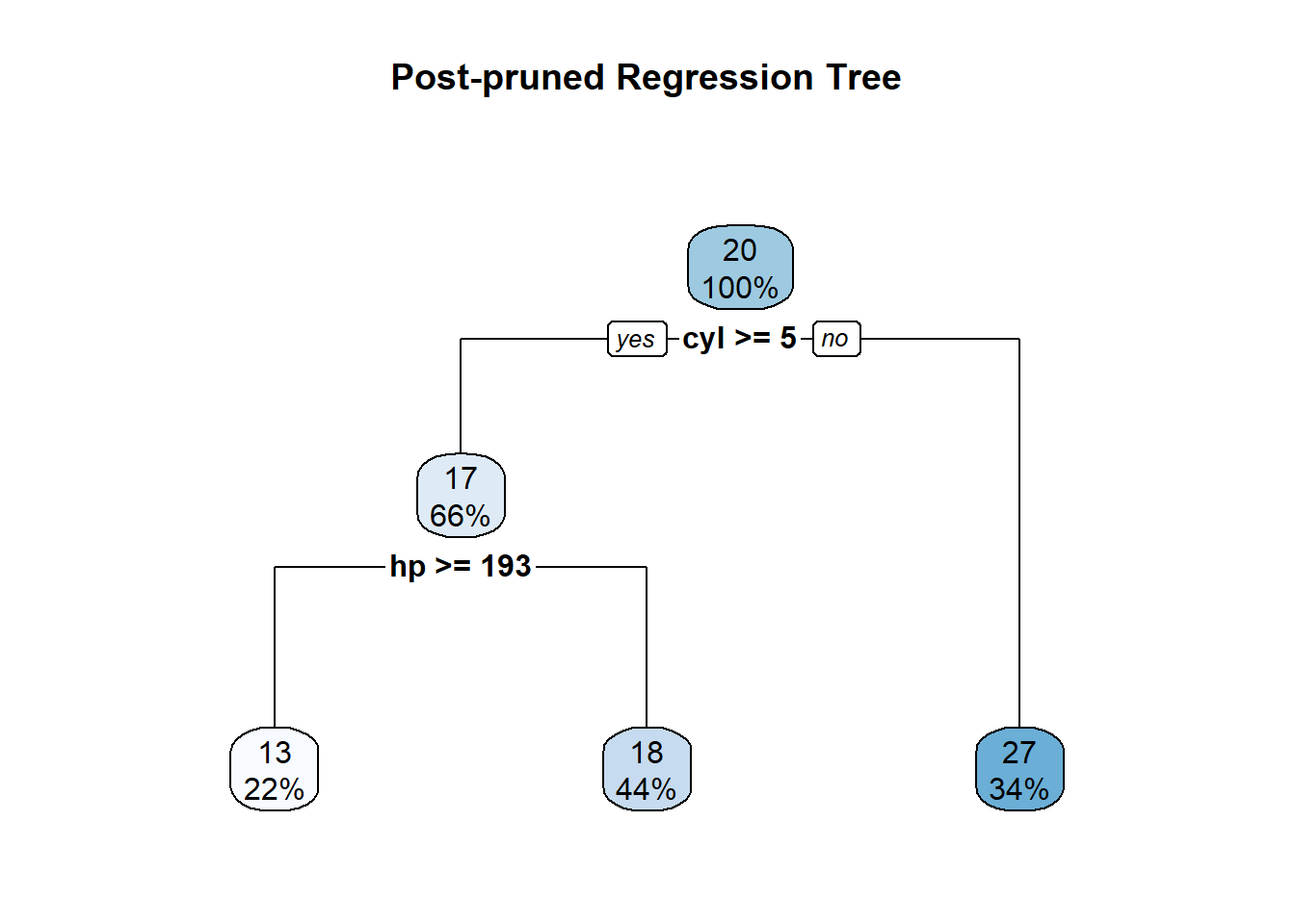

# Step 7: Summarize pruned model
summary(pruned_tree)

Call:
rpart(formula = mpg ~ ., data = mtcars, method = "anova", control = rpart.control(cp = 1e-04))
  n= 32 

          CP nsplit rel error    xerror      xstd
1 0.64312523      0 1.0000000 1.0260596 0.2455202
2 0.09748407      1 0.3568748 0.6474280 0.1694045
3 0.00010000      2 0.2593907 0.5381142 0.1213682

Variable importance
 cyl disp   hp   wt qsec   vs carb 
  20   20   19   16   12   11    1 

Node number 1: 32 observations,    complexity param=0.6431252
  mean=20.09062, MSE=35.18897 
  left son=2 (21 obs) right son=3 (11 obs)
  Primary splits:
      cyl  < 5      to the right, improve=0.6431252, (0 missing)
      wt   < 2.3925 to the right, improve=0.6356630, (0 missing)
      disp < 163.8  to the right, improve=0.6130502, (0 missing)
      hp   < 118    to the right, improve=0.6010712, (0 missing)
      vs   < 0.5    to the left,  improve=0.4409477, (0 missing)
  Surrogate splits:
      disp < 142.9  to the right, agree=0.969, adj=0.909, (0 split)
      hp   < 101    to the right, agree=0.938, adj=0.818, (0 split)
      wt   < 2.5425 to the right, agree=0.906, adj=0.727, (0 split)
      qsec < 18.41  to the left,  agree=0.844, adj=0.545, (0 split)
      vs   < 0.5    to the left,  agree=0.844, adj=0.545, (0 split)

Node number 2: 21 observations,    complexity param=0.09748407
  mean=16.64762, MSE=9.451066 
  left son=4 (7 obs) right son=5 (14 obs)
  Primary splits:
      hp   < 192.5  to the right, improve=0.5530828, (0 missing)
      cyl  < 7      to the right, improve=0.5068475, (0 missing)
      disp < 266.9  to the right, improve=0.5068475, (0 missing)
      wt   < 3.49   to the right, improve=0.4414890, (0 missing)
      drat < 3.075  to the left,  improve=0.1890739, (0 missing)
  Surrogate splits:
      disp < 334    to the right, agree=0.857, adj=0.571, (0 split)
      wt   < 4.66   to the right, agree=0.810, adj=0.429, (0 split)
      qsec < 15.455 to the left,  agree=0.810, adj=0.429, (0 split)
      carb < 3.5    to the right, agree=0.762, adj=0.286, (0 split)
      gear < 4.5    to the right, agree=0.714, adj=0.143, (0 split)

Node number 3: 11 observations
  mean=26.66364, MSE=18.48959 

Node number 4: 7 observations
  mean=13.41429, MSE=4.118367 

Node number 5: 14 observations
  mean=18.26429, MSE=4.276582

3.10 Classification Trees: Best Split, Entropy, and Gini Coefficients

Classification trees are used when the response variable is categorical.
At each node, the algorithm tries to find the best split — the one that produces the most homogeneous (pure) child nodes.

3.10.1 The Idea of “Best Split”

At any node in the tree:

The data are divided into two (or more) groups based on a predictor.
The best split is the one that makes each resulting group as pure as possible with respect to the class labels.

To measure purity, we use impurity measures such as:

Entropy
Gini index
(Sometimes) Misclassification error

3.10.2 Entropy

Entropy measures the disorder or uncertainty in a node.

If there are ( K ) classes and ( p_k ) is the proportion of observations belonging to class ( k ), then:

\[ \text{Entropy} = - \sum_{k=1}^{K} p_k \log_2(p_k) \]

3.10.2.1 Properties:

Entropy = 0 → Node is perfectly pure (all observations belong to one class).
Entropy is maximum when all classes are equally likely.

3.10.2.2 Example:

Class	Count	\(p_k\)	\(-p_k \log_2(p_k)\)
A	8	0.8	0.257
B	2	0.2	0.464

\[ \text{Entropy} = 0.257 + 0.464 = 0.721 \]

3.10.3 Gini Index

The Gini coefficient (or Gini impurity) is another measure of node impurity.

\[ \text{Gini} = 1 - \sum_{k=1}^{K} p_k^2 \]

3.10.3.1 Properties:

Gini = 0 → Perfectly pure node
Gini is smaller when the node is more homogeneous

3.10.3.2 Example:

Using the same proportions as above ( \(p_1 = 0.8, p_2 = 0.2\) ):

\[ \text{Gini} = 1 - (0.8^2 + 0.2^2) = 1 - (0.64 + 0.04) = 0.32 \]

3.10.4 Misclassification Error (less common)

A simpler impurity measure sometimes used:

\[ \text{Error} = 1 - \max(p_k) \]

For the same node ( \(\max(p_k) = 0.8\) ):

\[ \text{Error} = 1 - 0.8 = 0.2 \]

3.10.5 Choosing the Best Split

For each possible split:

Compute the impurity (Entropy or Gini) before splitting — call this \(I_{\text{parent}}\).
Compute the impurity of the child nodes (weighted by their sizes):

\[ I_{\text{split}} = \frac{n_L}{n} I_L + \frac{n_R}{n} I_R \]

Compute the information gain (reduction in impurity):

\[ \text{Gain} = I_{\text{parent}} - I_{\text{split}} \]

The best split is the one that maximizes this gain (i.e., gives the largest reduction in impurity).

3.10.6 Comparing Entropy and Gini

Property	Entropy	Gini
Range	0 to 1	0 to 0.5
Shape	Logarithmic	Quadratic
Interpretation	Information theory measure	Probability of misclassification
Behavior	Slightly more sensitive to rare classes	Computationally simpler
Commonly used in	C4.5, ID3 algorithms	CART algorithm

Both criteria often lead to similar splits in practice.