Exercise 3 Matrices, Arrays, Data frames
3.1 Lecture slides
3.2 Matrices
Use the code below to create the vector uniform.values.
set.seed(21)
uniform.values <- runif(50)
uniform.values
[1] 0.78611493 0.25244560 0.69925230 0.18446075 0.95961383 0.91868340
[7] 0.10180455 0.17219168 0.98600368 0.84939610 0.66754012 0.93521022
[13] 0.05818433 0.61861583 0.17491846 0.03767539 0.52531317 0.28218425
[19] 0.49904520 0.63382510 0.01139965 0.60785656 0.77559853 0.92397118
[25] 0.29170673 0.78907624 0.56849721 0.77843508 0.71323253 0.66904867
[31] 0.93470991 0.50646019 0.74506019 0.83835263 0.86907475 0.19311168
[37] 0.21633194 0.65042346 0.33516604 0.50765589 0.65283937 0.96557667
[43] 0.51466067 0.06165677 0.15101646 0.63556589 0.10296050 0.77269430
[49] 0.41022537 0.87023337- Arrange data in
uniform.valuesaccording to the following formats:
single row matrix.
single column matrix
matrix \(5 \times 10\)
matrix \(10 \times 5\)
- Write the code to output the following matrix.
       [,1]      [,2]      [,3]      [,4]      [,5]      [,6]      [,7]
a 0.7861149 0.2524456 0.6992523 0.1844608 0.9596138 0.9186834 0.1018046
b 0.7890762 0.5684972 0.7784351 0.7132325 0.6690487 0.9347099 0.5064602
       [,8]      [,9]     [,10]     [,11]     [,12]      [,13]     [,14]
a 0.1721917 0.9860037 0.8493961 0.6675401 0.9352102 0.05818433 0.6186158
b 0.7450602 0.8383526 0.8690747 0.1931117 0.2163319 0.65042346 0.3351660
      [,15]      [,16]     [,17]     [,18]      [,19]     [,20]      [,21]
a 0.1749185 0.03767539 0.5253132 0.2821842 0.49904520 0.6338251 0.01139965
b 0.5076559 0.65283937 0.9655767 0.5146607 0.06165677 0.1510165 0.63556589
      [,22]     [,23]     [,24]     [,25]
a 0.6078566 0.7755985 0.9239712 0.2917067
b 0.1029605 0.7726943 0.4102254 0.8702334- Matrix visualization: The matrix
mcontains 70 randomly generated values from the \(Unif(0, 1)\) distribution. The R functionimageis used to visualize the matrix.
set.seed(1)
values <- runif(70)
m <- matrix(values, 10, 7)
m
[,1] [,2] [,3] [,4] [,5] [,6] [,7]
[1,] 0.26550866 0.2059746 0.93470523 0.4820801 0.8209463 0.47761962 0.91287592
[2,] 0.37212390 0.1765568 0.21214252 0.5995658 0.6470602 0.86120948 0.29360337
[3,] 0.57285336 0.6870228 0.65167377 0.4935413 0.7829328 0.43809711 0.45906573
[4,] 0.90820779 0.3841037 0.12555510 0.1862176 0.5530363 0.24479728 0.33239467
[5,] 0.20168193 0.7698414 0.26722067 0.8273733 0.5297196 0.07067905 0.65087047
[6,] 0.89838968 0.4976992 0.38611409 0.6684667 0.7893562 0.09946616 0.25801678
[7,] 0.94467527 0.7176185 0.01339033 0.7942399 0.0233312 0.31627171 0.47854525
[8,] 0.66079779 0.9919061 0.38238796 0.1079436 0.4772301 0.51863426 0.76631067
[9,] 0.62911404 0.3800352 0.86969085 0.7237109 0.7323137 0.66200508 0.08424691
[10,] 0.06178627 0.7774452 0.34034900 0.4112744 0.6927316 0.40683019 0.87532133image(m, useRaster=TRUE, axes=FALSE)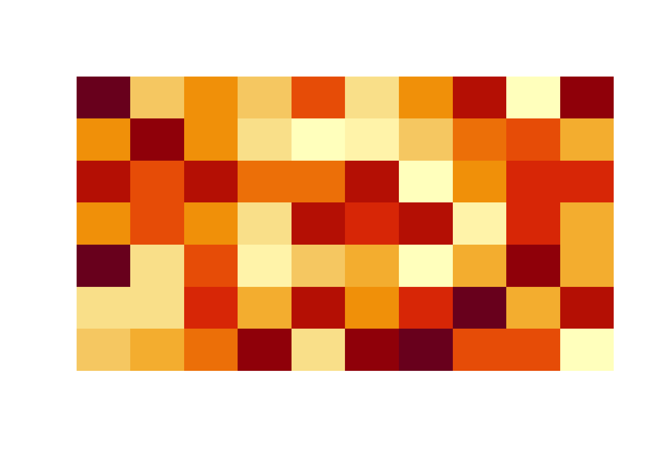
Record the values in the matrix (m) as follows: matrix value = 0 if value lessthan 0.5 and 1 otherwise. Write an R code to visualize the new matrix.
Consider the matrix
ymatgiven below. Convert all even index position values to 0 and odd position values to 1.
      [,1] [,2] [,3] [,4] [,5] [,6] [,7] [,8] [,9] [,10]
 [1,]   10  110  210  310  410  510  610  710  810   910
 [2,]   20  120  220  320  420  520  620  720  820   920
 [3,]   30  130  230  330  430  530  630  730  830   930
 [4,]   40  140  240  340  440  540  640  740  840   940
 [5,]   50  150  250  350  450  550  650  750  850   950
 [6,]   60  160  260  360  460  560  660  760  860   960
 [7,]   70  170  270  370  470  570  670  770  870   970
 [8,]   80  180  280  380  480  580  680  780  880   980
 [9,]   90  190  290  390  490  590  690  790  890   990
[10,]  100  200  300  400  500  600  700  800  900  1000
Help:
5 %% 2[1] 16 %% 2[1] 0- Visualize the resulted matrix using the
imagefunction. Your output should look like this:

3.3 Array
- Write R codes to create the following arrays.
, , Matrix1

     COL1 COL2 COL3
ROW1    1   10   13
ROW2    2   11   14
ROW3    3   12   15

, , Matrix2

     COL1 COL2 COL3
ROW1    1   10   13
ROW2    2   11   14
ROW3    3   12   15
, , 1
[,1] [,2] [,3]
[1,] 2 4 6
[2,] 3 5 7
, , 2
[,1] [,2] [,3]
[1,] 8 10 12
[2,] 9 11 133.4 List
- Create a list store the built-in dataset
irisdataset and “scatterplot ofSepal.WidthandSepal.Length.”
3.5 Dataframe
There are several datasets, which comes with R installation. For example iris, mtcars and ,any more. In this exercise we will work with the mtcars dataset in R.You may refer to the help page ?mtcars for more details about the dataset.
Use suitable R functions for quick exploration of data. Help:
str,head,tail,dim,nrow,ncol.What happens when you call
View()onmtcars?Write an R code to extract column names and row names.
Extract and display the column corresponding to the number of cylinders.
Extract and display the observations of cars with 4 cylinders AND 4 gears.
What is the maximum
mpg?Which car has the maximum
mpg?Compute suitable summary statistics for each column.