4 Random Forests
4.1 Decision trees - Limitation
To capture a complex decision boundary we need to use a deep tree
In-class explanation
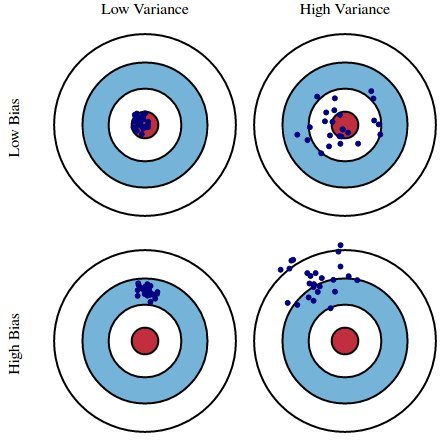
4.2 Bias-Variance Trade off
- A deep decision tree has low bias and high variance.
4.3 Bagging (Bootstrap Aggregation)
Technique for reducing the variance of an estimated predicted function
Works well for high-variance, low-bias procedures, such as trees
4.4 Ensemble Methods
Combines several base models
Bagging (Bootstrap Aggregation) is an ensemble method
4.5 Ensemble Methods
“Ensemble learning gives credence to the idea of the “wisdom of crowds,” which suggests that the decision-making of a larger group of people is typically better than that of an individual expert.”
4.6 Bootstrap
- Generate multiple samples of training data, via bootstrapping
Example
Training data: \(\{(y_1, x_1), (y_2, x_2), (y_3, x_3), (y_4, x_4)\}\)
Three samples generated from bootstrapping
Sample 1 = \(\{(y_1, x_1), (y_2, x_2), (y_3, x_3), (y_4, x_4)\}\)
Sample 2 = \(\{(y_1, x_1), (y_1, x_1), (y_1, x_1), (y_4, x_4)\}\)
Sample 3 = \(\{(y_1, x_1), (y_2, x_2), (y_1, x_1), (y_4, x_4)\}\)
4.7 Aggregation
Train a decision tree on each bootstrap sample of data without pruning.
Aggregate prediction using either voting or averaging
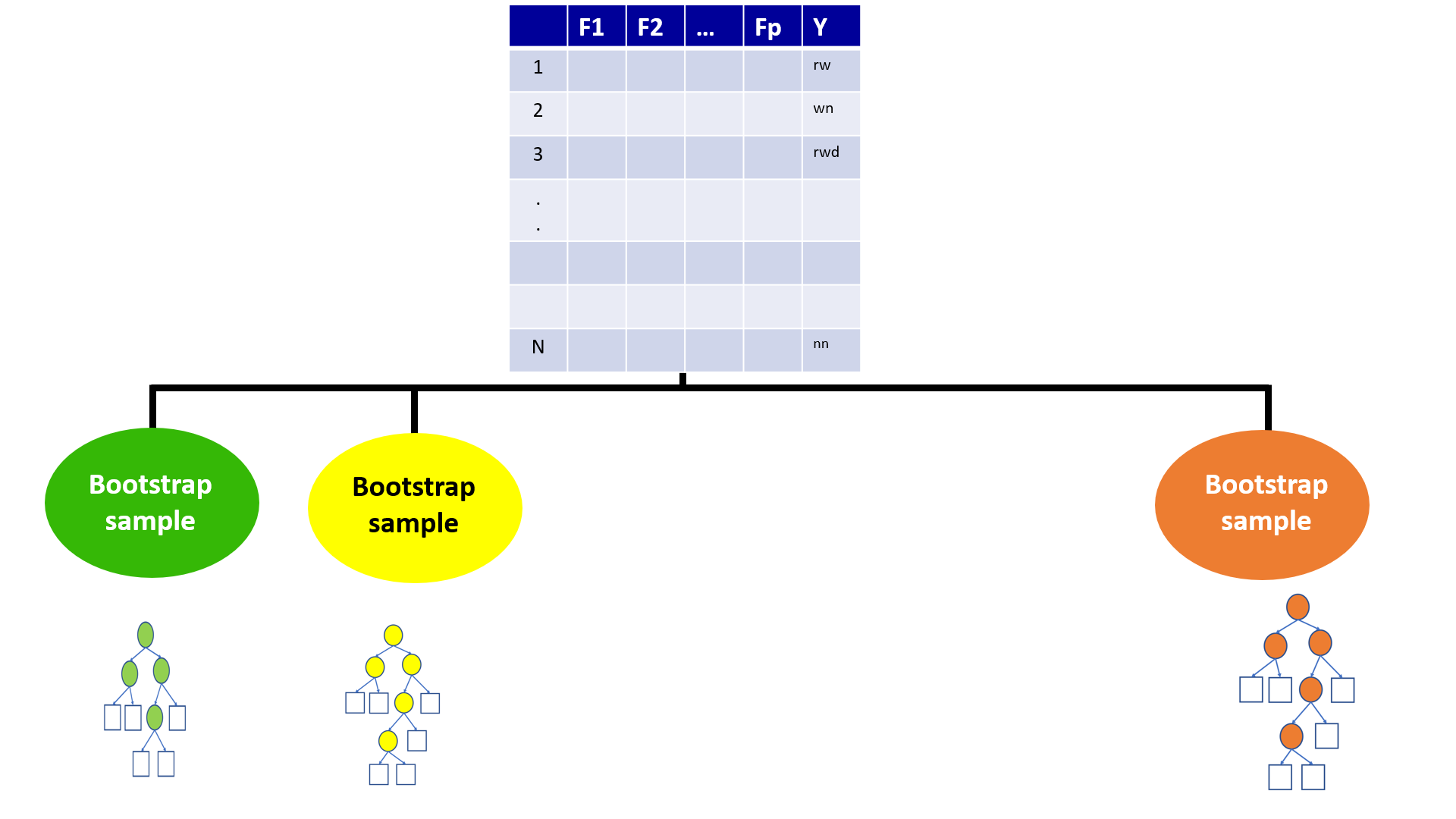
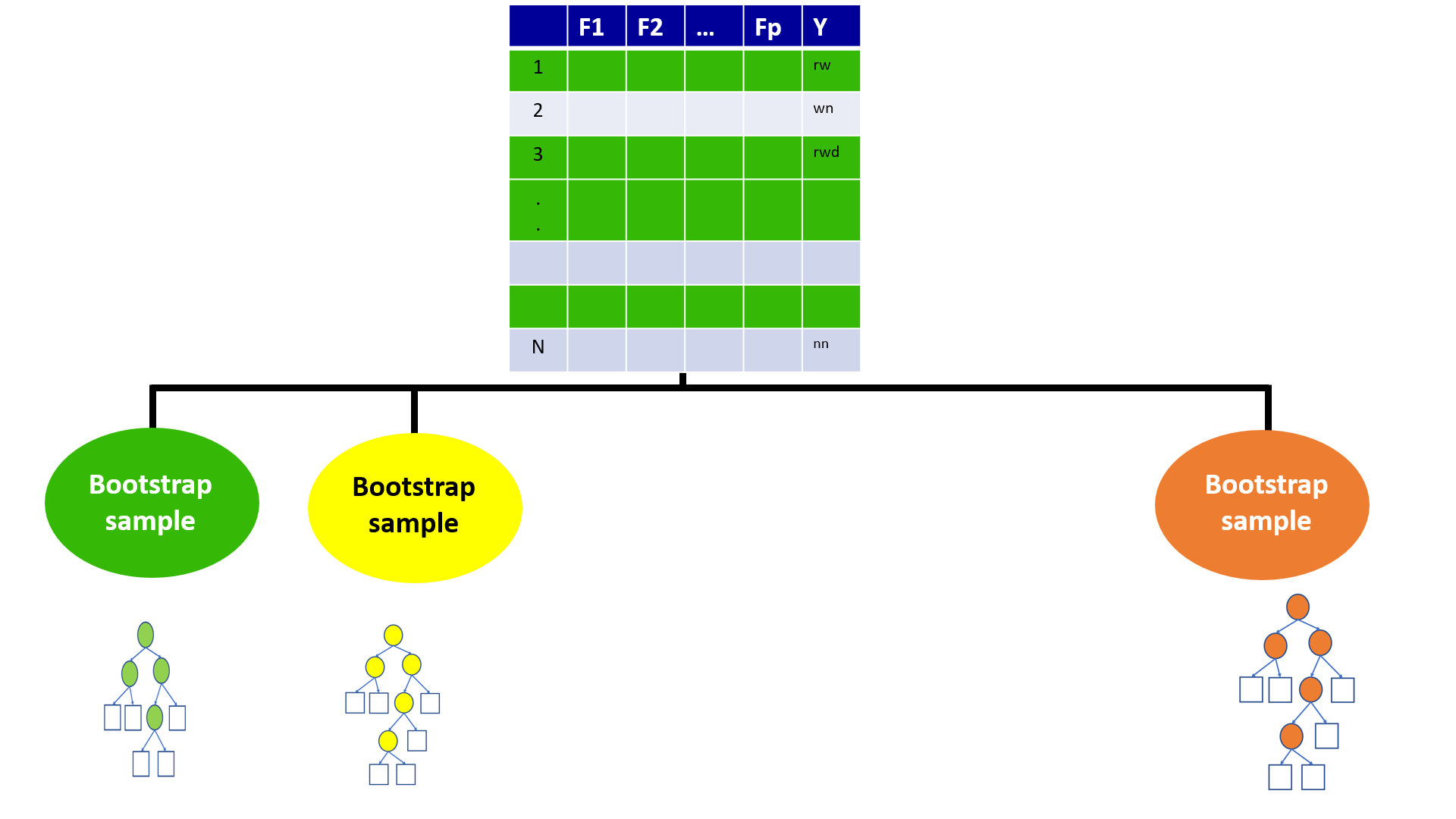
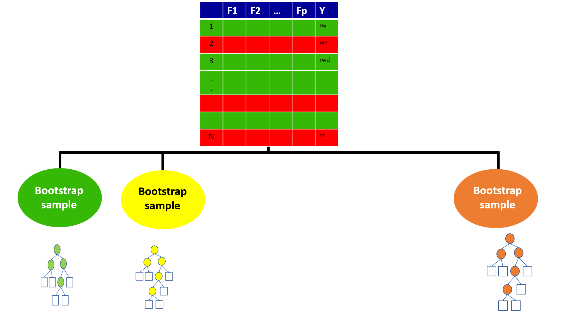
4.8 Bagging - in class diagram
4.9 Bagging
Pros
Ease of implementation
Reduction of variance
Cons
Loss of interpretability
Computationally expensive
4.10 Bagging
Bootstrapped subsamples are created
A Decision Tree is formed on each bootstrapped sample.
The results of each tree are aggregated
4.11 Random Forests: Improving on Bagging
The ensembles of trees in Bagging tend to be highly correlated.
All of the bagged trees will look quite similar to each other. Hence, the predictions from the bagged trees will be highly correlated.
4.12 Random Forests
Bootstrap samples
At each split, randomly select a set of predictors from the full set of predictors
From the selected predictors we select the optimal predictor and the optimal corresponding threshold for the split.
Grow multiple trees and aggregate
4.13 Random Forests - Hyper parameters
Number of variables randomly sampled as candidates at each split
Number of trees to grow
Minimum size of terminal nodes. Setting this number larger causes smaller trees to be grown (and thus take less time).
Note: In theory, each tree in the random forest is full (not pruned), but in practice this can be computationally expensive,thus, imposing a minimum node size is not unusual.
4.14 Random Forests
Bagging ensemble method
Gives final prediction by aggregating the predictions of bootstrapped decision tree samples.
Trees in a random forest are independent of each other.
4.15 Random Forests
Pros
- Accuracy
Cons
Speed
Interpretability
Overfitting
4.16 Out-of-bag error
With ensemble methods, we get a new metric for assessing the predictive performance of the model, the out-of-bag error
4.17 Random Forests
4.18 Random Forests
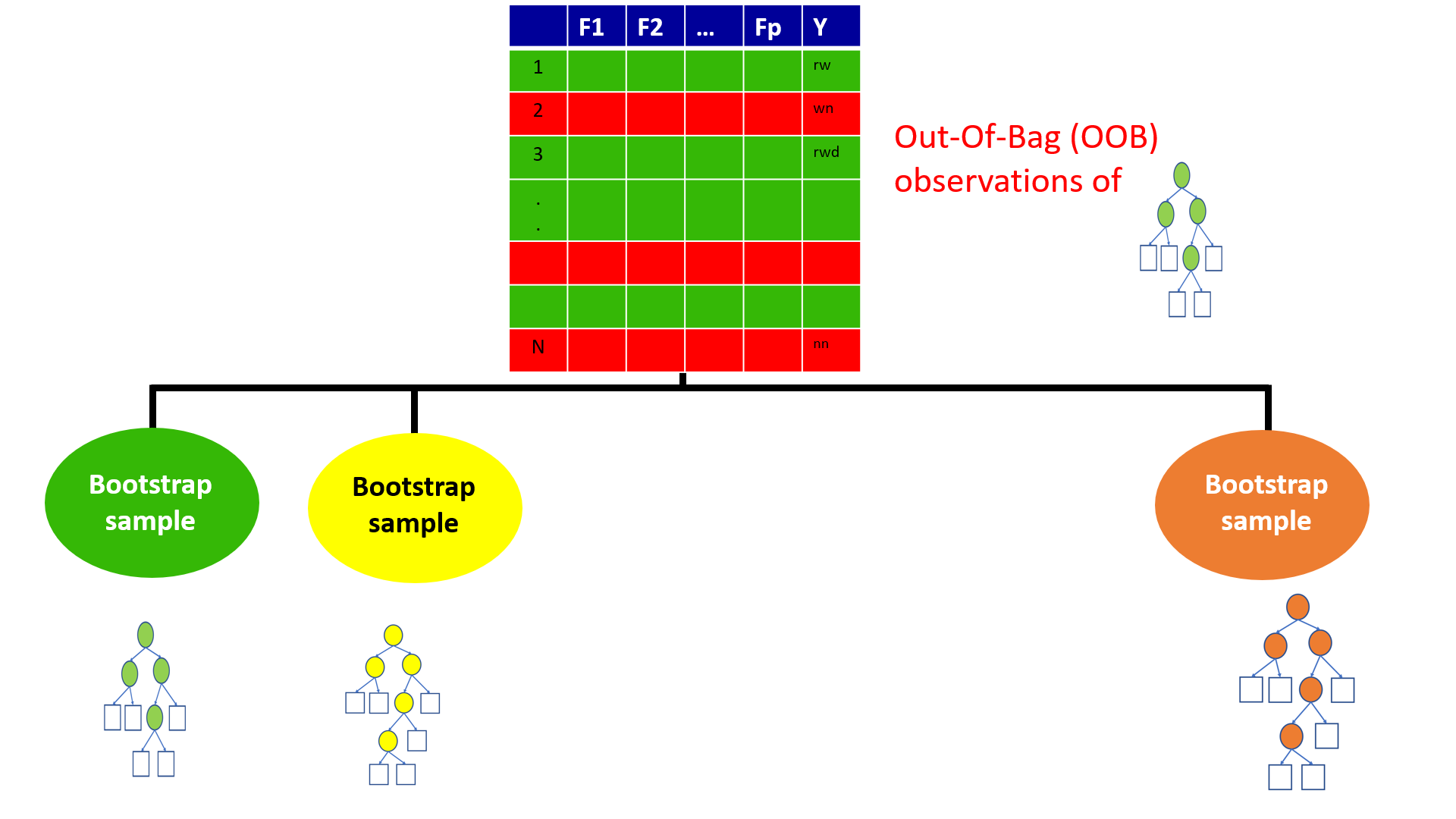
4.19 Out-of-Bag (OOB) Samples
4.20 Out-of-Bag (OOB) Samples
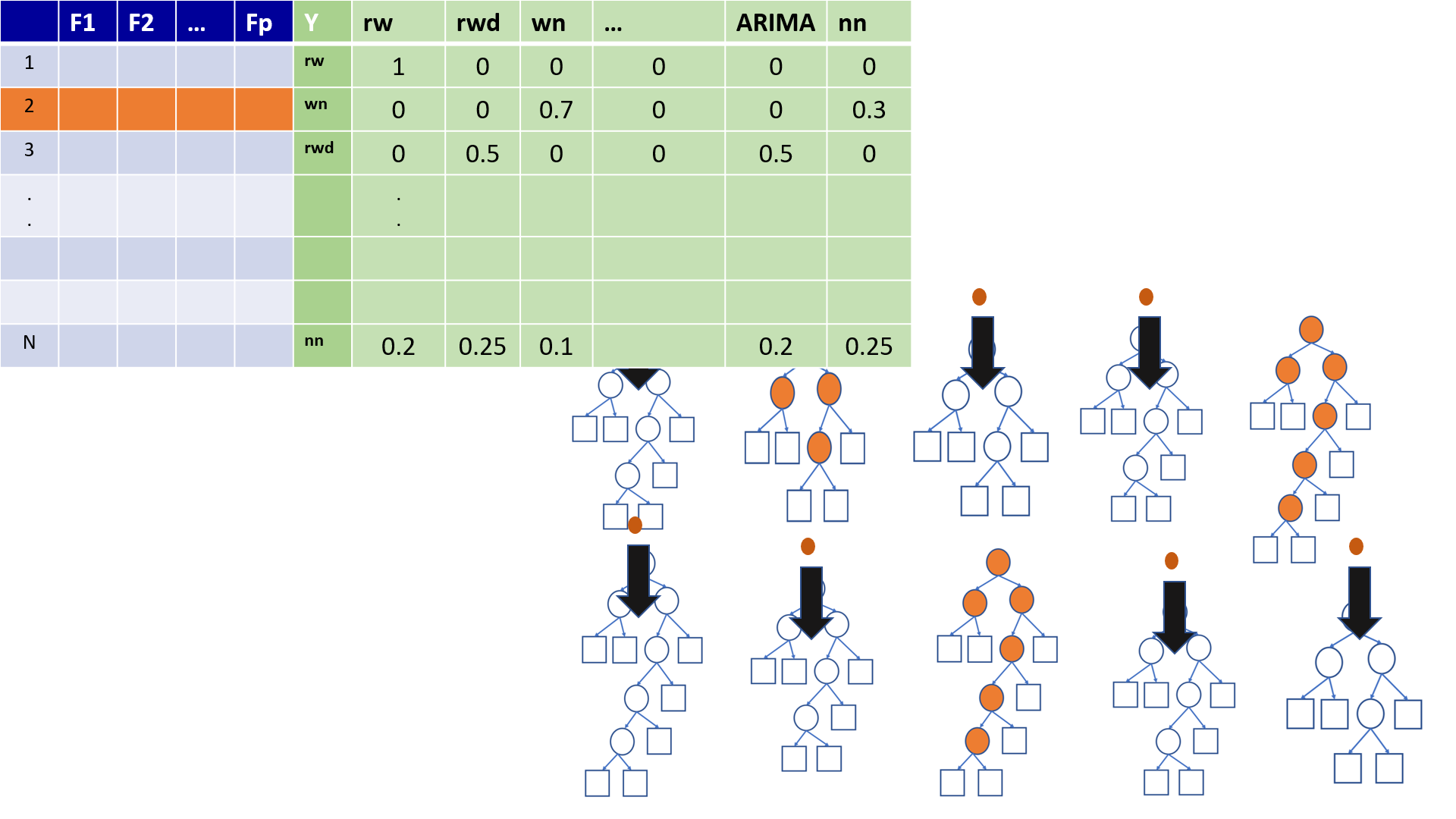
4.21 Predictions based on OOB observations
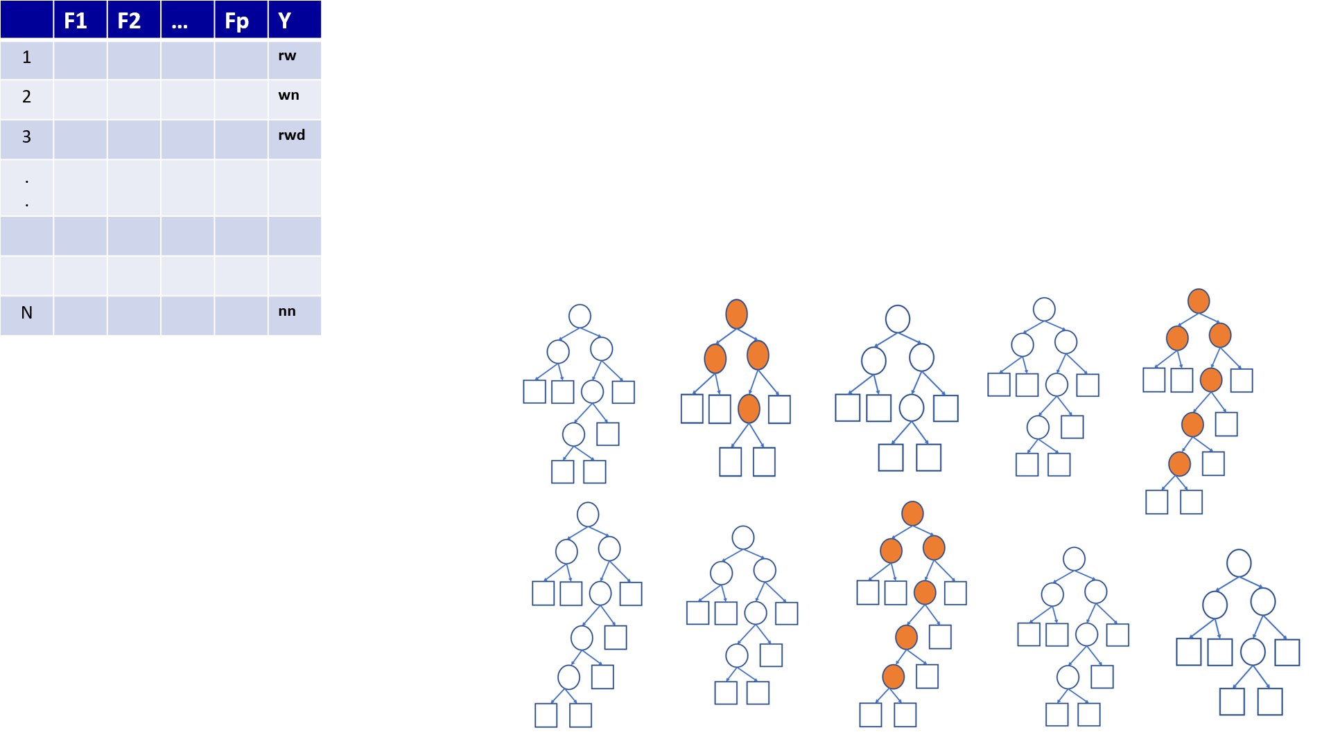
4.22 Predictions based on OOB observations
Figure 1
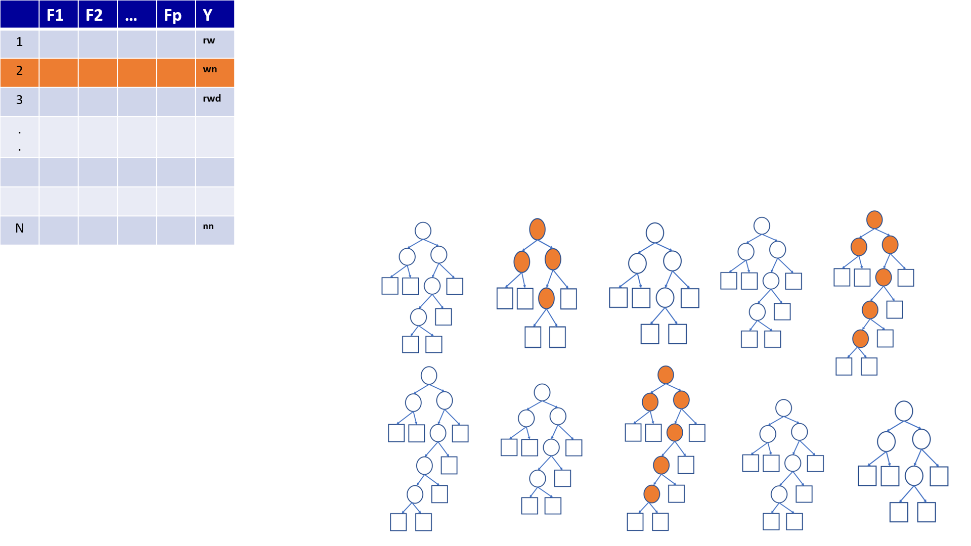
Figure 2
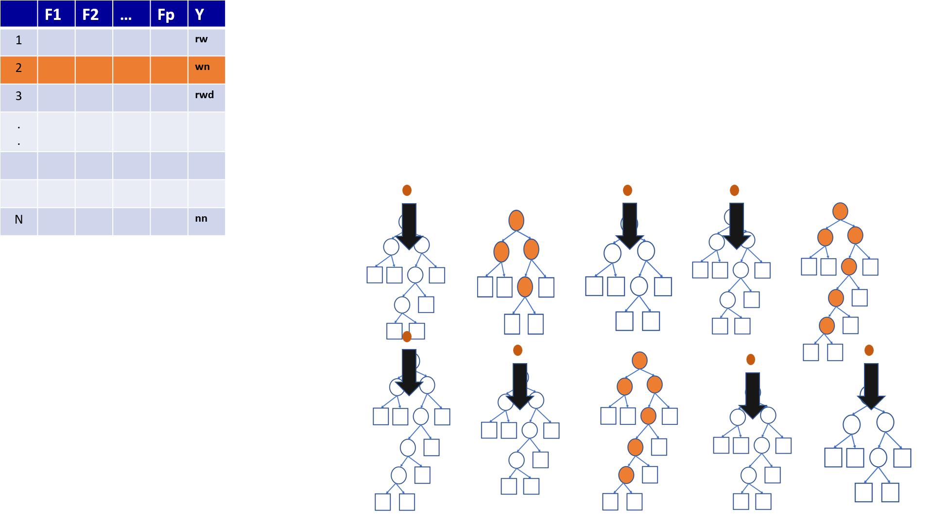
Figure 3
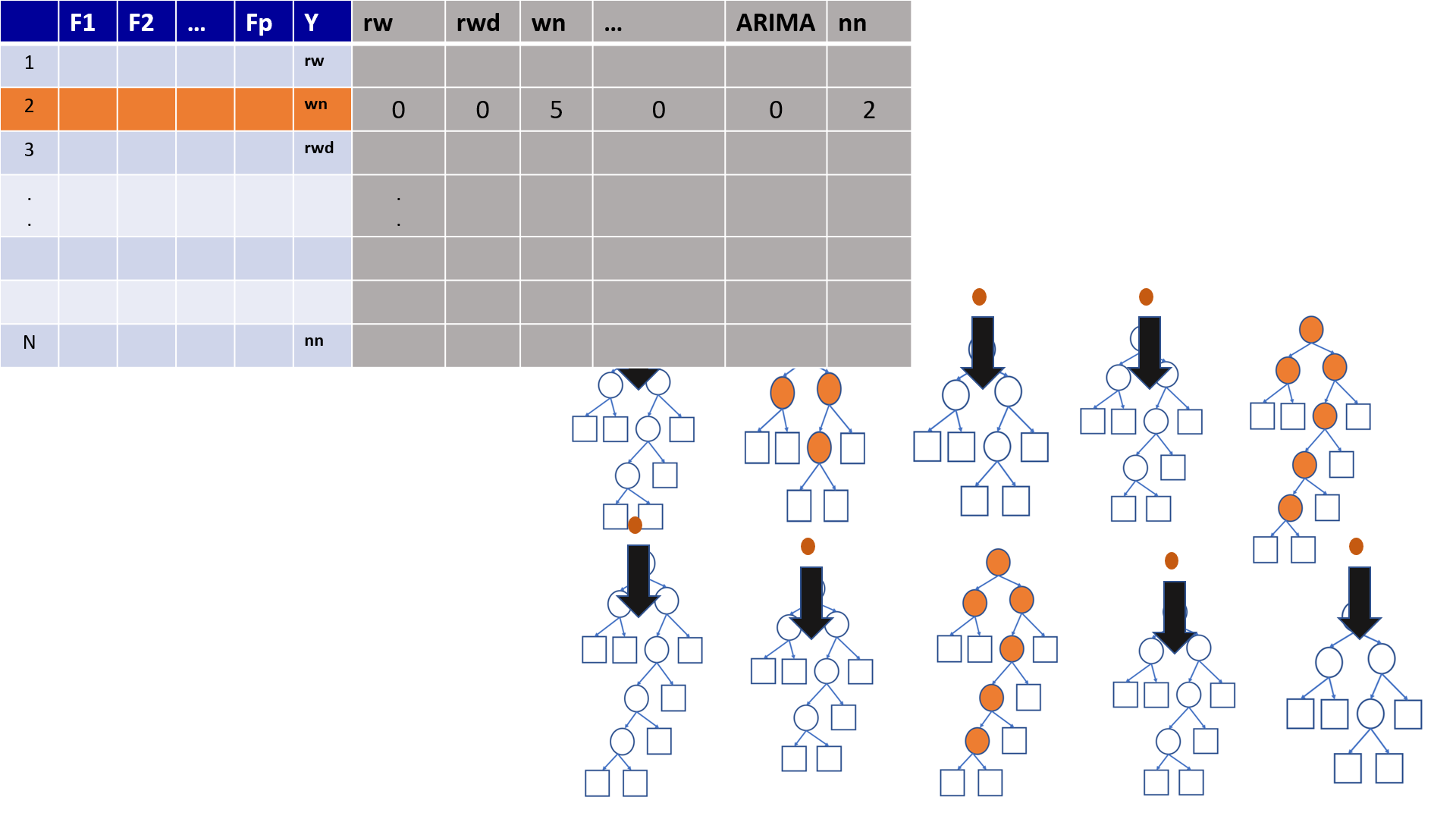
Figure 4

Figure 5

Figure 6
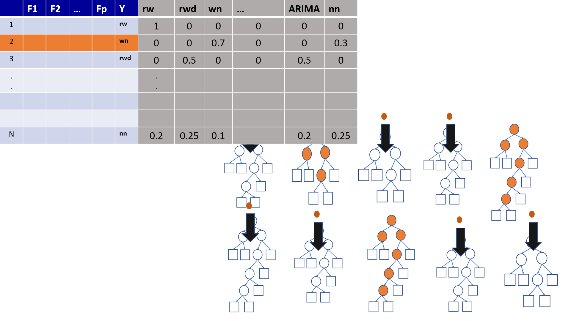
Figure 7
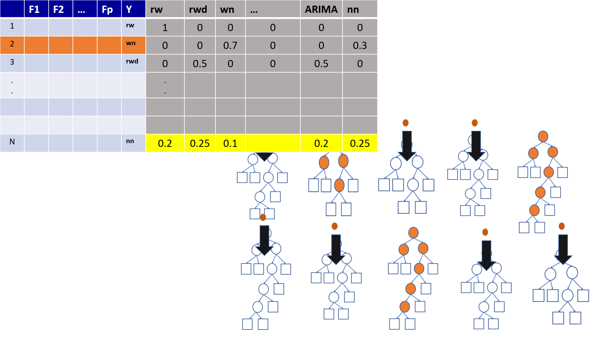
Figure 8
4.23 Variable Importance in Random Forest
contribution to predictive accuracy
Permutation-based variable importance
Mean decrease in Gini coefficient
4.24 Permutation-based variable importance
the OOB samples are passed down the tree, and the prediction accuracy is recorded
the values for the \(j^{th}\) variable are randomly permuted in the OOB samples, and the accuracy is again computed.
the decrease in accuracy as a result of this permuting is averaged over all trees, and is used as a measure of the importance of variable \(j\) in the random forests
4.25 Mean decrease in Gini coefficient
Measure of how each variable contributes to the homogeneity of the nodes and leaves in the resulting random forest
The higher the value of mean decrease accuracy or mean decrease Gini score, the higher the importance of the variable in the model
4.26 Boosting
Bagging and boosting are two main types of ensemble learning methods.
The main difference between bagging and boosting is the way in which they are trained.
In bagging, weak learners (decision trees) are trained in parallel, but in boosting, they learn sequentially.
4.27 Boosting
Fit a single tree
Draw a sample that gives higher selection probabilities to misclassified records
Fit a tree to the new sample
Repeat Steps 2 and 3 multiple times
Use weighted voting to classify records, with heavier weights for later trees
4.28 Boosting
Iterative process.
Each tree is dependent on the previous one. Hence, it is hard to parallelize the training process of boosting algorithms.
The training time will be higher. This is the main drawback of boosting algorithms.
4.29 Boosting Algorithms
Adaptive boosting or AdaBoost
Gradient boosting
Extreme gradient boosting or XGBoost