9 Support Vector Machine

9.1 What is a hyperplane?

A hyperplane is a flat, dividing surface in a vector space that’s one dimension smaller than the space it’s in; it generalizes concepts like lines (in 2D) and planes (in 3D) to higher dimensions, acting as a decision boundary in machine learning for separating data into classes.

In-class

Hyperplane in 2D
Hyperplane in 3D

Reading

9.2 Mathematical Definition of Hyperplanes

In-class

9.3 Classification Using a Separating Hyperplane

One can easily determine on which side of the hyperplane a point lies by simply calculating the sign.

9.4 There can be multiple number of hyperplanes. Which is the best?

In-class diagram

9.5 Criteria for choosing the best hyperplane

Maximum margin (SVM approach):

Pick the hyperplane where the distance to the nearest points on both sides is maximized.

Ensures better generalization.
Minimizing classification error:

Count the number of misclassified points for each hyperplane.

Choose the hyperplane with the fewest misclassifications.
Other metrics (if regression or probabilistic separation):

Accuracy, Precision, Recall, F1-score for classification.

Mean Squared Error (MSE) for regression.

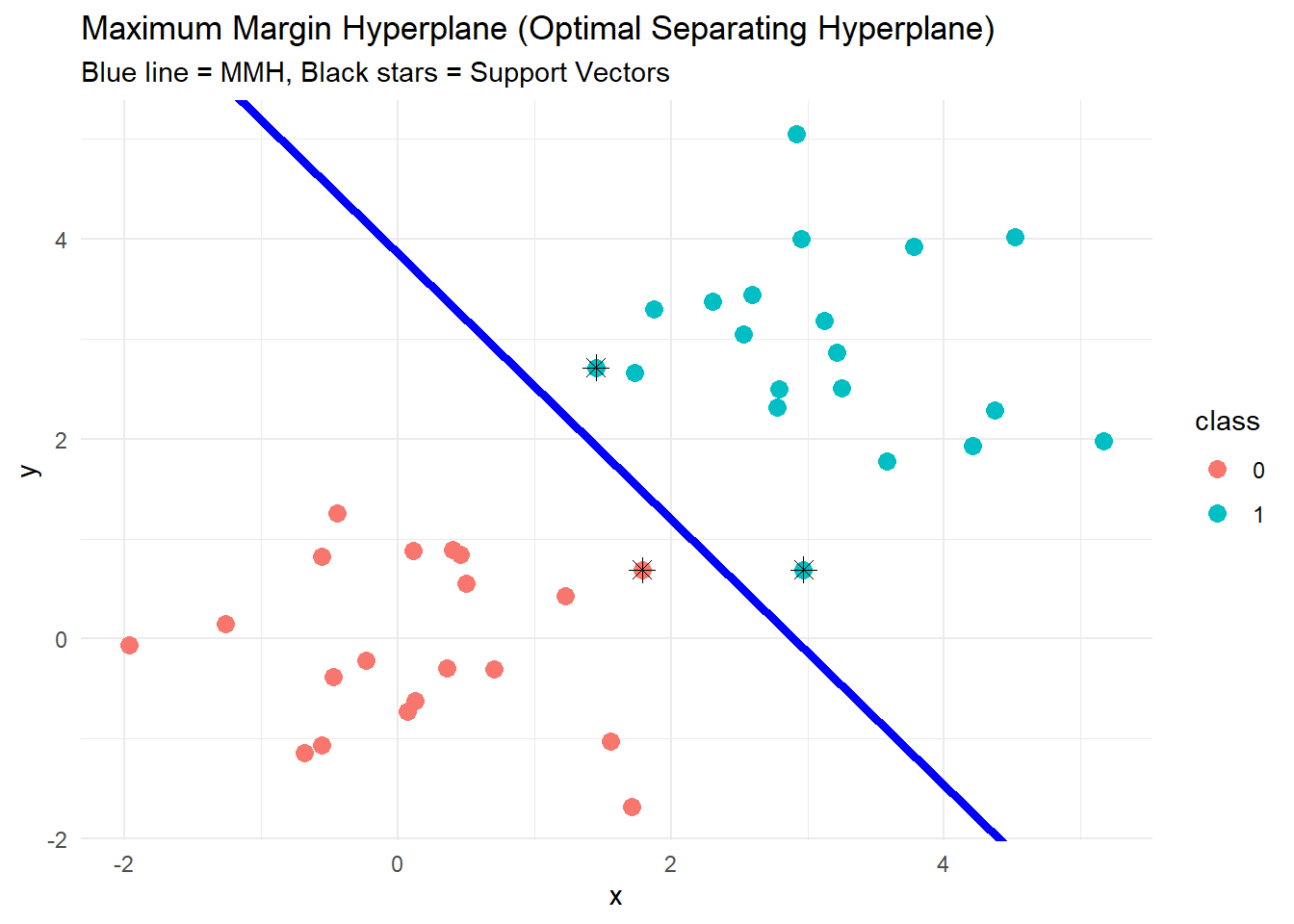
9.6 Maximal Margin Hyperplane (Optimal Separating Hyperplane)

Concept:

For linearly separable data:

There are many hyperplanes that can separate two classes.

The maximum margin hyperplane is the one that maximizes the distance (margin) to the nearest points of both classes.

Imagine a 2D scenario:

You have two groups of points on a piece of paper:

Group A (e.g., red dots)

Group B (e.g., green dots)

You want to draw a straight line that separates the two groups.

There are many possible lines that can separate them.

The “maximum margin” idea:

Instead of just picking any line, you want the line to be as far away as possible from the nearest points in each group.

Why?

This gives more “breathing room” for your decision.

Makes the classification more robust to new points or slight noise.

The distance between the line and the nearest points of each group is called the margin.

The Maximum Margin Hyperplane is the line that makes this margin as wide as possible.

Simple analogy:

Think of a road between two rows of parked cars:

There’s many possible paths you could drive through.

You choose the path that keeps the largest distance from both rows, so you have maximum safety space.

That “safest path” is like the maximum margin hyperplane.

9.7 Maximal Margin Hyperplane: Optimization problem

In-class

Reading

9.8 Limitations: Maximal Margin Hyperplane

Sensitive to outliers

Example: One point far away from its class can completely change the hyperplane.

Since the MMH tries to maximize margin while keeping all points correctly classified, even a single outlier may force the hyperplane to tilt badly.

This can reduce the generalization to new data.
Cannot handle non-linearly separable data

If the two classes overlap, there is no hyperplane that separates them perfectly.

Hard-margin SVM cannot be applied directly in this case.
Overfitting risk

If we try to force perfect separation with noisy data, the MMH may fit very tightly to specific points, which is not robust.

9.9 Soft margin classifier or Support Vector Classifier (SVC)

Like the Maximum Margin Classifier (MMC), the main goal of the Support Vector Classifier (SVC) is to find the best boundary that separates classes. However, unlike the MMC, which needs a perfect separation, the SVC allows a few points to be misclassified. This makes it more flexible and robust, especially when the data is noisy or the classes overlap.

9.10 Support Vector Classifier: Optimization Problem

In-class

9.11 Support Vector Machine (SVM): Kernel Trick (Non-linear boundary)

Sometimes, the classes in your data cannot be separated by a straight line (not linearly separable).
The kernel trick lets SVM draw a straight line in a higher-dimensional space, which corresponds to a curved or non-linear boundary in the original space.

In other words

Start simple in low dimensions. If the data cannot be separated, lift it to a higher-dimensional space. Then find the widest possible road (support vector classifier) that separates the classes, allowing some flexibility if needed.

Diagrams

9.12 Summary

A Support Vector Machine (SVM) is a supervised machine learning algorithm used for classification and regression. Its main goal is to find the best boundary (hyperplane) that separates different classes of data.

For linearly separable data: SVM finds the Maximum Margin Hyperplane (MMH), which maximizes the distance to the nearest points of each class.

For real-world or noisy data: SVM uses a soft margin (Support Vector Classifier) to allow some misclassifications while still maximizing the margin.

For non-linear separation: SVM can use kernels to transform the data into a higher-dimensional space where a linear boundary can separate classes.

9.13 SVM with R

9.13.1 Example 1

Data

# Small dataset
df <- data.frame(
  x = c(1, 2, 3, 4, 5, 6),
  y = c(2, 1, 4, 5, 4, 6),
  class = factor(c(0, 0, 0, 1, 1, 1))
)

df

  x y class
1 1 2     0
2 2 1     0
3 3 4     0
4 4 5     1
5 5 4     1
6 6 6     1

Fit SVM

library(e1071)
# Fit linear SVM
svm_model <- svm(class ~ x + y, data = df, kernel = "linear", cost = 1)
# Print model summary
summary(svm_model)


Call:
svm(formula = class ~ x + y, data = df, kernel = "linear", cost = 1)


Parameters:
   SVM-Type:  C-classification 
 SVM-Kernel:  linear 
       cost:  1 

Number of Support Vectors:  5

 ( 3 2 )


Number of Classes:  2 

Levels: 
 0 1

Predictions

# Predict on training data
pred <- predict(svm_model, df)

# Compare predictions with true labels
df$pred <- pred
df

  x y class pred
1 1 2     0    0
2 2 1     0    0
3 3 4     0    1
4 4 5     1    1
5 5 4     1    1
6 6 6     1    1

Accuracy Measures

# Confusion matrix
table(Predicted = df$pred, Actual = df$class)

         Actual
Predicted 0 1
        0 2 0
        1 1 3

# Accuracy
accuracy <- mean(df$pred == df$class)
accuracy

[1] 0.8333333

9.13.2 Example 2

# Loading necessary libraries
library(e1071)
library(ggplot2)

# Preparing data
data(iris)
subset_iris <- iris[iris$Species != 'setosa', c(1, 2, 5)]

# Building SVM model
svm_model <- svm(Species~., data = subset_iris, method="C-classification", 
                 kernel = "linear")

# Plotting with base R
plot(svm_model, subset_iris)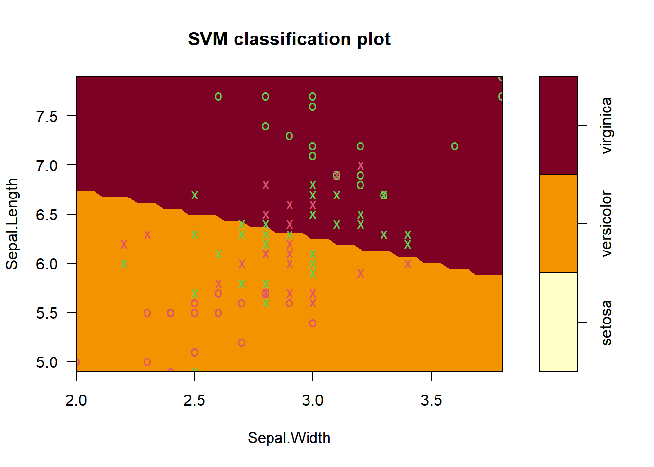

svm_data <- data.frame(subset_iris, fit=predict(svm_model, subset_iris))
ggplot(svm_data, aes(y=Sepal.Length, x=Sepal.Width, color=Species)) +
    geom_point() +
    geom_point(data=svm_data[svm_model$index,], aes(y=Sepal.Length, x=Sepal.Width), 
               shape=8, size=3) +
    labs(title="SVM Classification with ggplot2")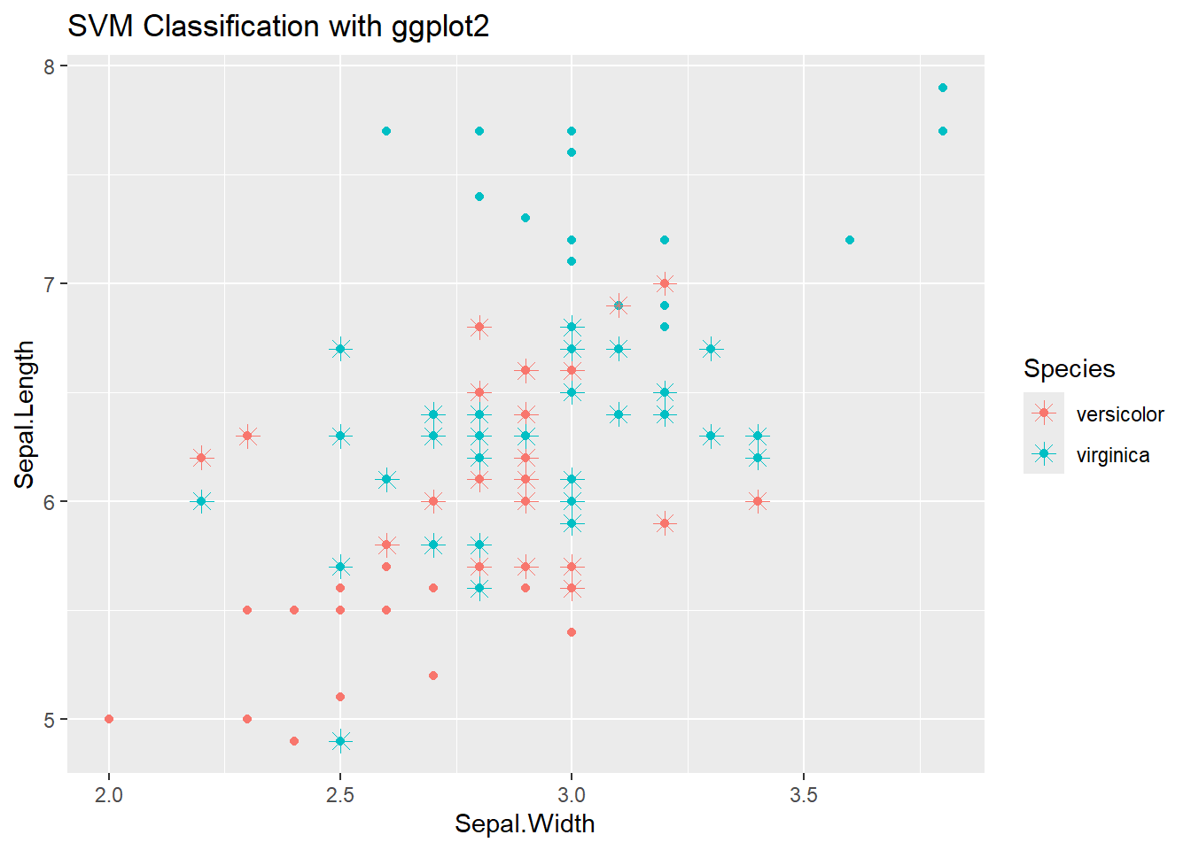

When you train an SVM model in R using the e1071::svm() function, the algorithm tries to find the optimal hyperplane that separates the classes. Not all points in your dataset influence this hyperplane — only some of them lie on the margin or are close to it. These critical points are called support vectors. svm_model$index contains the row numbers (indices) of the training data that are support vectors. These support vectors are the only points that define the SVM decision boundary. Points far from the margin do not affect the hyperplane.

9.14 Multi-class classification using Support Vector Machines

Support Vector Machines (SVMs) are inherently binary classifiers designed to find an optimal hyperplane separating two classes. To adapt SVMs for multi-class classification (problems with three or more classes), the problem is typically decomposed into multiple binary classification tasks using specific strategies.

The two most common methods for achieving multi-class classification with SVMs are:

1. One-vs-Rest (OvR) or One-vs-All (OvA)

In the OvR approach, a separate binary SVM model is trained for each class.

Training Phase: If there are (N) classes, (N) different SVM classifiers are trained. For classifier (i), all instances of class (i) are treated as positive examples, and all instances from the other (N-1) classes are grouped together as negative examples.Prediction Phase: For a new data point, all (N) classifiers run their predictions. The classifier that outputs the highest score or confidence determines the final class label.

Pros/Cons: This method is computationally efficient in training as it only requires fitting (N) models. However, it can suffer from class imbalance because the “rest” class is usually much larger than the single “one” class. It’s often preferred when computational efficiency is a priority.

2. One-vs-One (OvO)

The OvO method trains a binary SVM for every possible pair of classes. For (N) classes, this means training (N*(N-1)/2) classifiers, each using data only from the two classes it is trained to distinguish. During prediction, each classifier votes for one of its two classes, and the data point is assigned to the class with the most votes. OvO is more computationally intensive in training than OvR but can offer higher accuracy through focused pairwise comparisons. It scales well with the number of training samples but not as well with a large number of classes.

9.15 SVM Hyper Parameters

C (Cost)

Purpose: Regularization parameter controlling the trade-off between training accuracy and model generalization.

Effect:

Small C: Allows more misclassifications on the training data → wider margin → better generalization, less risk of overfitting.

Large C: Tries to classify all training examples correctly → narrower margin → risk of overfitting.

Intuition: Think of C as how “strict” the SVM is about classifying the training points correctly.
Kernel

Purpose: Transforms data into a higher-dimensional space so that it may become linearly separable.

Common kernels:

Linear: Use when data is already linearly separable.

Polynomial: Adds polynomial combinations of features; good for curved decision boundaries.

RBF (Gaussian): Maps data into infinite-dimensional space; popular default choice for non-linear problems.

Sigmoid: Similar to a neural network activation function; less commonly used.

Intuition: The kernel decides the “shape” of the decision boundary.
Gamma (γ)

Purpose: Defines how far the influence of a single training point reaches in the feature space.

Effect (RBF or polynomial kernels):

Low gamma: Each point has broad influence → smoother decision boundary → less risk of overfitting.

High gamma: Each point has very localized influence → more complex boundary → higher risk of overfitting.

Intuition: Think of gamma as how “far” each point can reach to affect the boundary.