8 Data Wrangling

8.1 Tidy Data

Each variable is placed in its column
Each observation is placed in its own row
Each value is placed in its own cell

8.1.1 Which data frames are tidy?

8.2 Reshaping data with tidyr

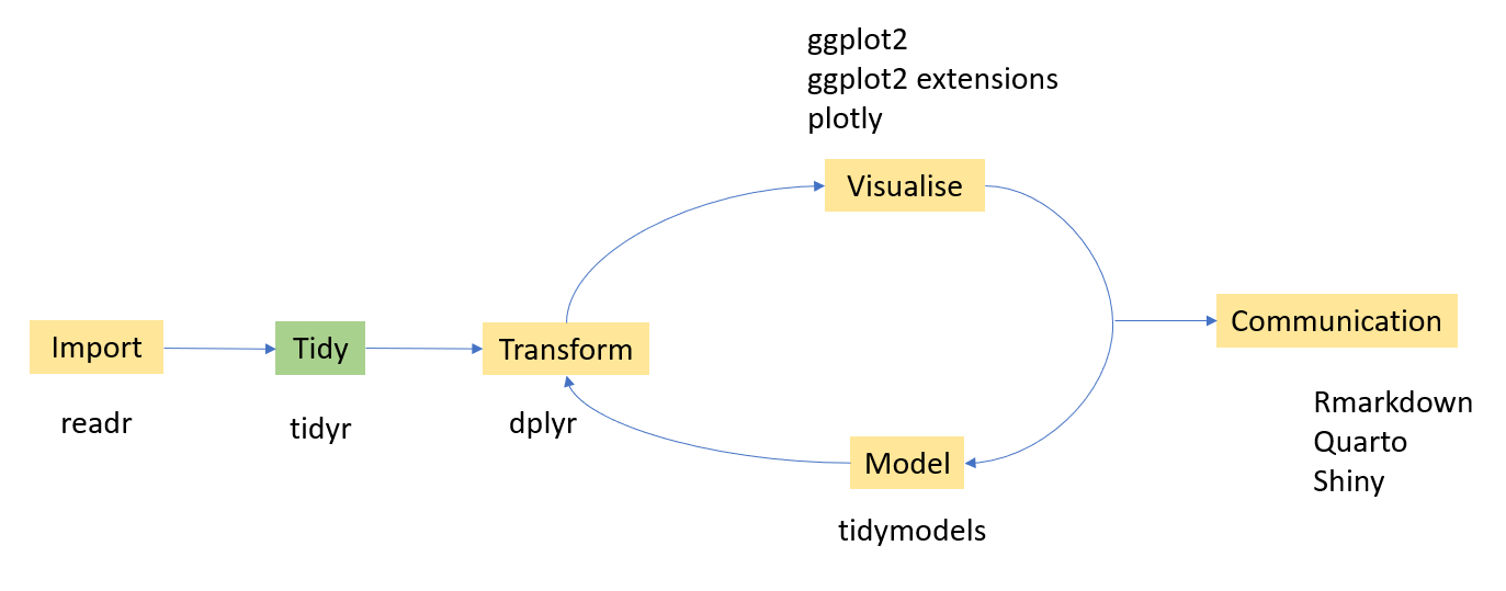
How to reshape your data in order to make the analysis easier?

We are going to learn four main functions in the tidyr package.

pivot_wider
pivot_longer
seperate
unite

Input and Output type for tidyr functions

Main input: data frame or tibble.

Output: tibble

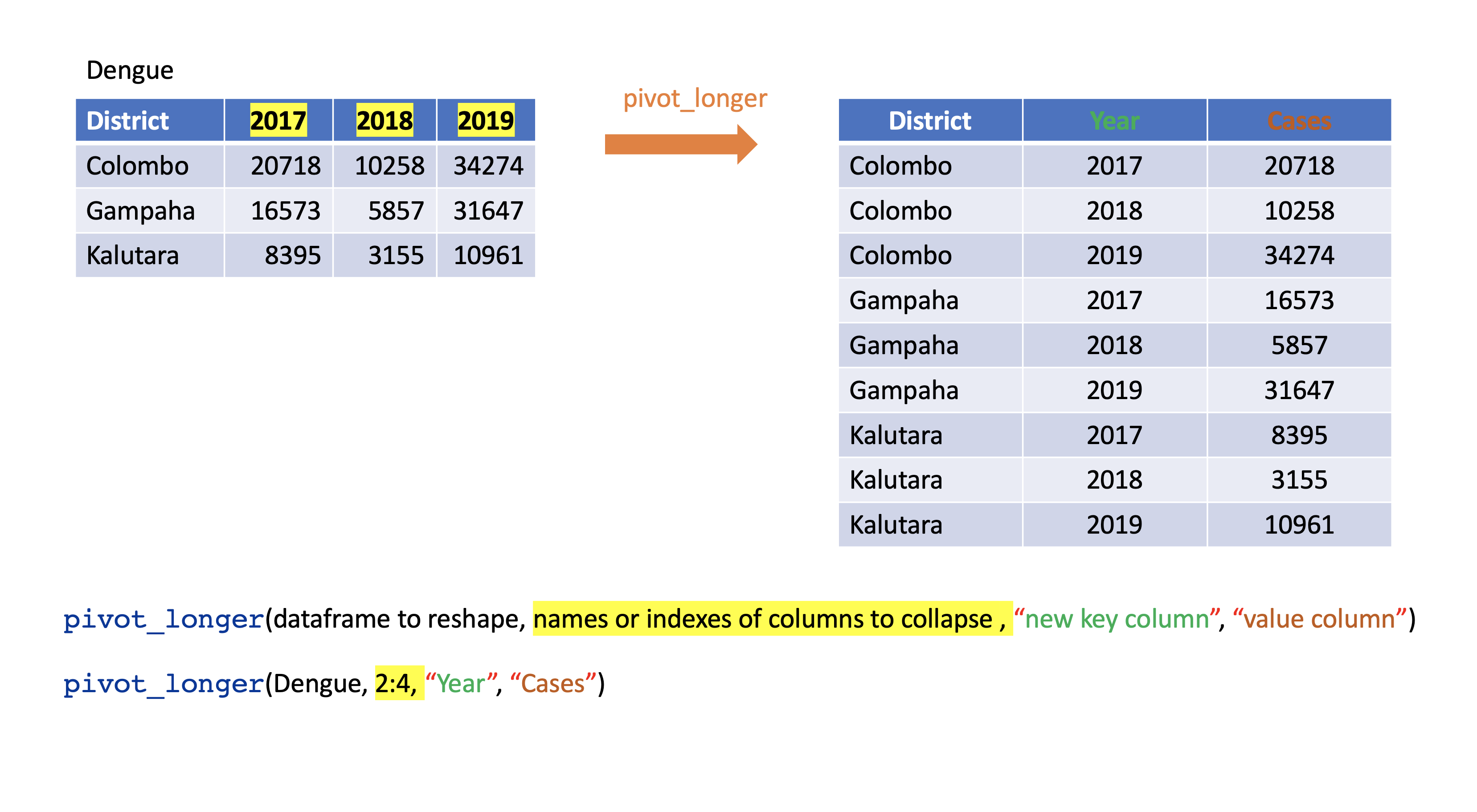
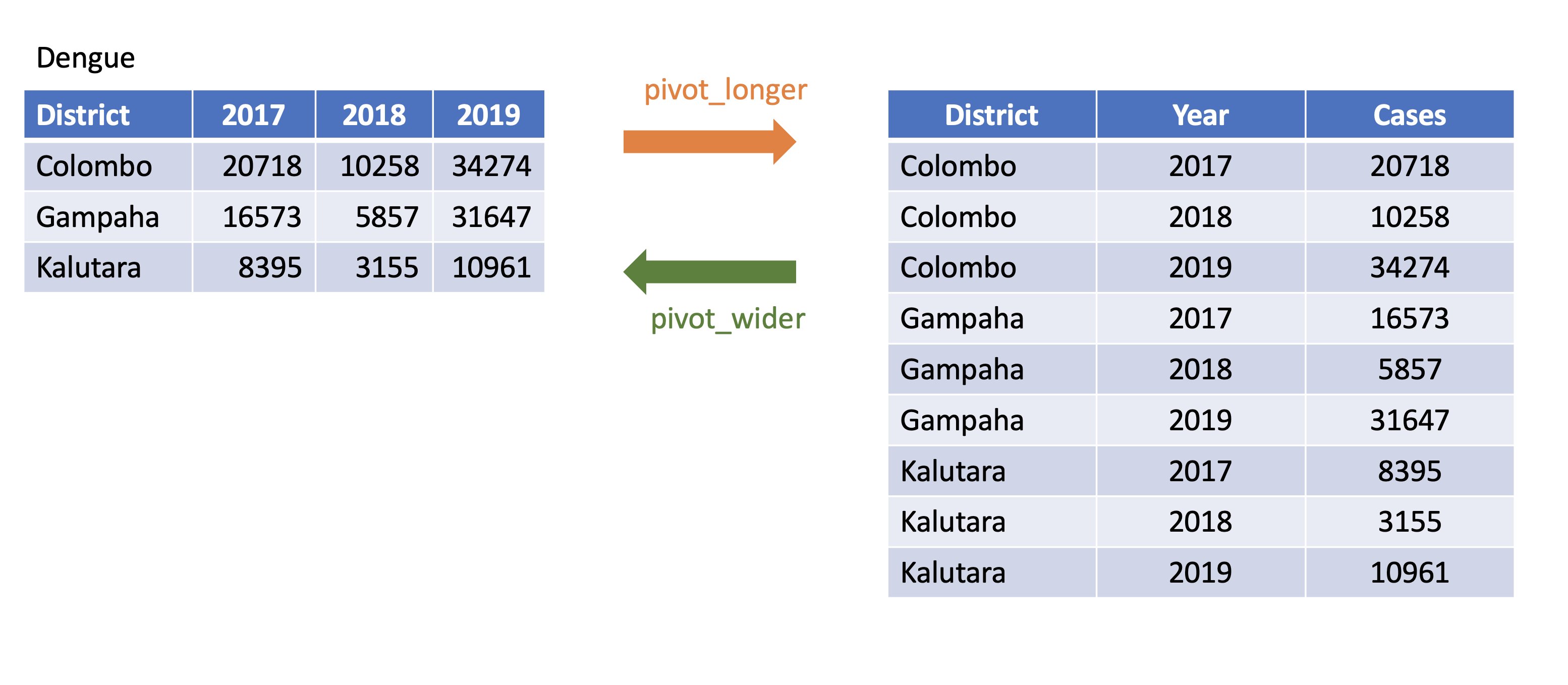
8.2.1 `pivot_longer()`

Turns columns into rows.
From wide format to long format.

library(tidyverse)
dengue <- tibble( dist = c("Colombo", "Gampaha", "Kalutara"), 
                  '2017' = c(20718, 10258, 34274), 
                  '2018' = c(16573, 5857, 31647), 
                  '2019' = c(8395, 3155, 10961)); 
dengue

# A tibble: 3 × 4
  dist     `2017` `2018` `2019`
  <chr>     <dbl>  <dbl>  <dbl>
1 Colombo   20718  16573   8395
2 Gampaha   10258   5857   3155
3 Kalutara  34274  31647  10961

dengue %>% 
  pivot_longer(2:4,
               names_to="Year", 
               values_to = "Dengue counts")

# A tibble: 9 × 3
  dist     Year  `Dengue counts`
  <chr>    <chr>           <dbl>
1 Colombo  2017            20718
2 Colombo  2018            16573
3 Colombo  2019             8395
4 Gampaha  2017            10258
5 Gampaha  2018             5857
6 Gampaha  2019             3155
7 Kalutara 2017            34274
8 Kalutara 2018            31647
9 Kalutara 2019            10961

8.2.2 `pivot_wider()`

From long to wide format.

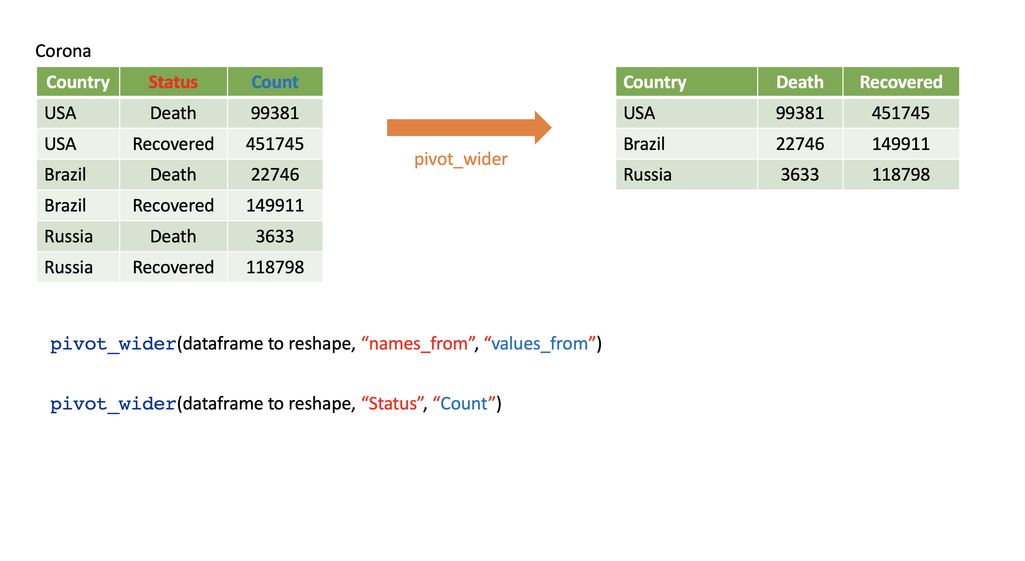
Corona <- tibble(
country = rep(c("USA", "Brazil", "Russia"), each=2),
status = rep(c("Death", "Recovered"), 3),
count = c(99381, 451745, 22746, 149911, 3633, 118798))

Corona

# A tibble: 6 × 3
  country status     count
  <chr>   <chr>      <dbl>
1 USA     Death      99381
2 USA     Recovered 451745
3 Brazil  Death      22746
4 Brazil  Recovered 149911
5 Russia  Death       3633
6 Russia  Recovered 118798

Corona %>% 
  pivot_wider(names_from=status, 
              values_from=count)

# A tibble: 3 × 3
  country Death Recovered
  <chr>   <dbl>     <dbl>
1 USA     99381    451745
2 Brazil  22746    149911
3 Russia   3633    118798

8.2.2.1 Assign a name to the new dataset

corona_wide_format <- Corona %>% 
  pivot_wider(names_from=status, 
              values_from=count)
corona_wide_format

# A tibble: 3 × 3
  country Death Recovered
  <chr>   <dbl>     <dbl>
1 USA     99381    451745
2 Brazil  22746    149911
3 Russia   3633    118798

8.2.2.2 `pivot_longer` vs `pivot_wider`

8.2.2.3 Dealing with missing values

# A tibble: 7 × 3
   year quarter income
  <dbl>   <dbl>  <dbl>
1  2015       1      2
2  2015       2     NA
3  2015       3      3
4  2015       4     NA
5  2016       2      4
6  2016       3      5
7  2016       4      6

profit %>%
pivot_wider(names_from = year, values_from = income)

# A tibble: 4 × 3
  quarter `2015` `2016`
    <dbl>  <dbl>  <dbl>
1       1      2     NA
2       2     NA      4
3       3      3      5
4       4     NA      6

Remove missing values

profit %>%
pivot_wider(names_from = year, values_from = income) %>%
pivot_longer(
cols = c(`2015`, `2016`),
names_to = "year",
values_to = "income",
values_drop_na = TRUE
)

# A tibble: 5 × 3
  quarter year  income
    <dbl> <chr>  <dbl>
1       1 2015       2
2       2 2016       4
3       3 2015       3
4       3 2016       5
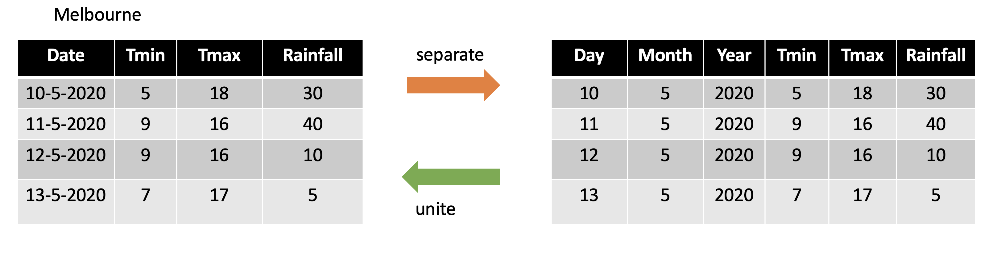
5       4 2016       6

8.2.3 `separate()`

Separate one column into several columns.

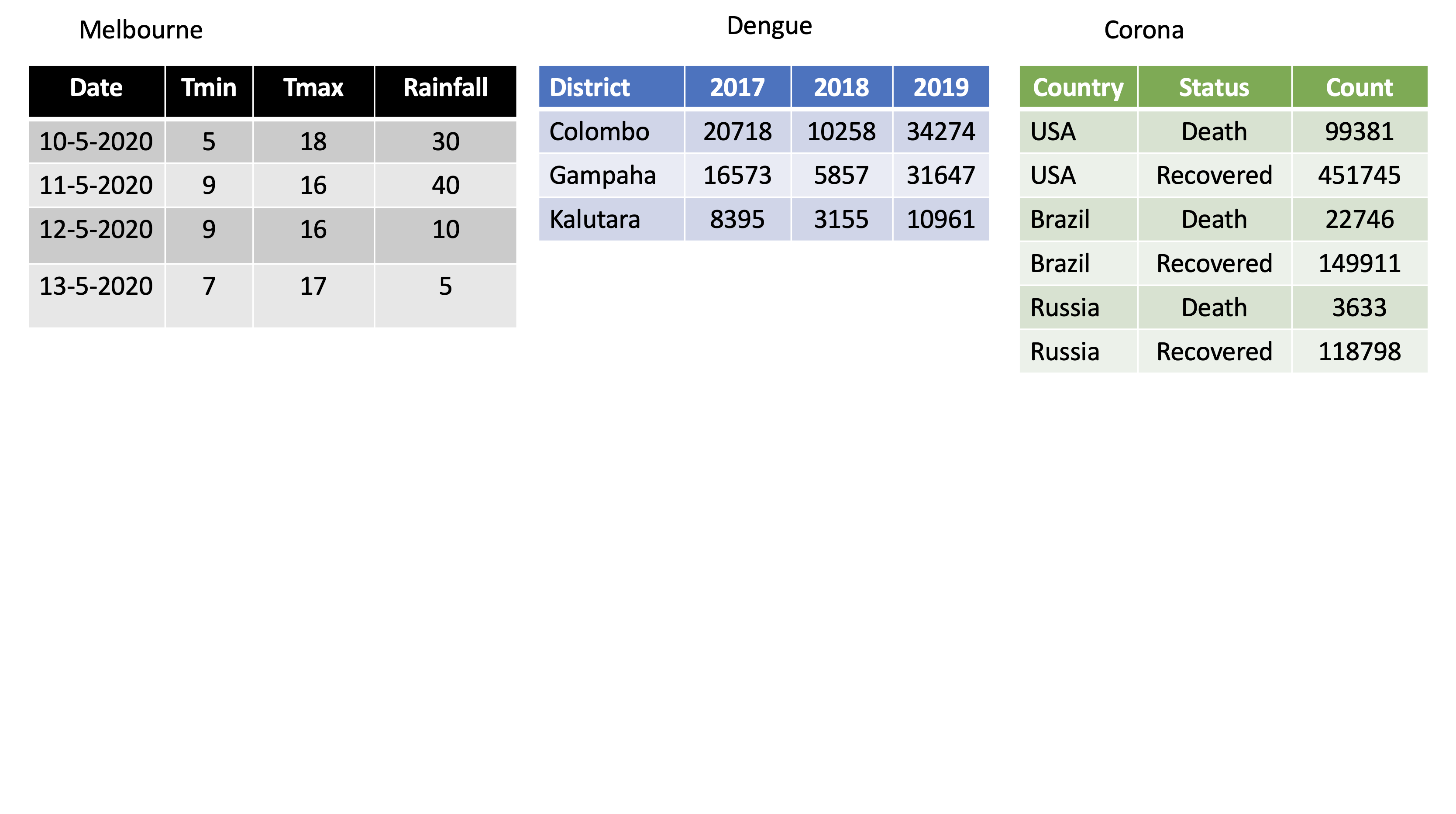
Melbourne <- 
  tibble(Date = c("10-5-2020", "11-5-2020", "12-5-2020","13-5-2020"),
         Tmin = c(5, 9, 9, 7), Tmax = c(18, 16, 16, 17),
         Rainfall= c(30, 40, 10, 5)); Melbourne

# A tibble: 4 × 4
  Date       Tmin  Tmax Rainfall
  <chr>     <dbl> <dbl>    <dbl>
1 10-5-2020     5    18       30
2 11-5-2020     9    16       40
3 12-5-2020     9    16       10
4 13-5-2020     7    17        5

Melbourne %>% separate(Date, into=c("day", "month", "year"), sep="-")

# A tibble: 4 × 6
  day   month year   Tmin  Tmax Rainfall
  <chr> <chr> <chr> <dbl> <dbl>    <dbl>
1 10    5     2020      5    18       30
2 11    5     2020      9    16       40
3 12    5     2020      9    16       10
4 13    5     2020      7    17        5

df <- data.frame(x = c(NA, "a.b", "a.d", "b.c"))
df

     x
1 <NA>
2  a.b
3  a.d
4  b.c

df %>% separate(x, c("Text1", "Text2"))

  Text1 Text2
1  <NA>  <NA>
2     a     b
3     a     d
4     b     c

tbl <- tibble(input = c("a", "a b", "a-b c", NA))
tbl

# A tibble: 4 × 1
  input
  <chr>
1 a    
2 a b  
3 a-b c
4 <NA>

tbl %>% 
  separate(input, c("Input1", "Input2"))

Warning: Expected 2 pieces. Additional pieces discarded in 1 rows [3].

Warning: Expected 2 pieces. Missing pieces filled with `NA` in 1 rows [1].

# A tibble: 4 × 2
  Input1 Input2
  <chr>  <chr> 
1 a      <NA>  
2 a      b     
3 a      b     
4 <NA>   <NA>

tbl <- tibble(input = c("a", "a b", "a-b c", NA)); tbl

# A tibble: 4 × 1
  input
  <chr>
1 a    
2 a b  
3 a-b c
4 <NA>

tbl %>% separate(input, c("Input1", "Input2", "Input3"))

Warning: Expected 3 pieces. Missing pieces filled with `NA` in 2 rows [1, 2].

# A tibble: 4 × 3
  Input1 Input2 Input3
  <chr>  <chr>  <chr> 
1 a      <NA>   <NA>  
2 a      b      <NA>  
3 a      b      c     
4 <NA>   <NA>   <NA>

8.2.4 `unite()`

Unite several columns into one.

projects <- tibble(
  Country = c("USA", "USA", "AUS", "AUS"),
  State = c("LA", "CO", "VIC", "NSW"),
  Cost = c(1000, 11000, 20000,30000)
)
projects

# A tibble: 4 × 3
  Country State  Cost
  <chr>   <chr> <dbl>
1 USA     LA     1000
2 USA     CO    11000
3 AUS     VIC   20000
4 AUS     NSW   30000

# A tibble: 4 × 3
  Country State  Cost
  <chr>   <chr> <dbl>
1 USA     LA     1000
2 USA     CO    11000
3 AUS     VIC   20000
4 AUS     NSW   30000

projects %>% unite("Location", c("State", "Country"))

# A tibble: 4 × 2
  Location  Cost
  <chr>    <dbl>
1 LA_USA    1000
2 CO_USA   11000
3 VIC_AUS  20000
4 NSW_AUS  30000

Specify the separator that you want to separate

projects %>% unite("Location", c("State", "Country"),
                   sep="-")

# A tibble: 4 × 2
  Location  Cost
  <chr>    <dbl>
1 LA-USA    1000
2 CO-USA   11000
3 VIC-AUS  20000
4 NSW-AUS  30000

8.2.4.1 `separate` vs `unite`

8.3 Data minipulation with `dplyr`

Under data manipulation with dplyr we will learn six main functions in the dplyr package. They are

filter
select
mutate
summarise
arrange
group_by
rename

8.3.1 Dataset used for demonstrations

library(gapminder)
str(gapminder)

tibble [1,704 × 6] (S3: tbl_df/tbl/data.frame)
 $ country  : Factor w/ 142 levels "Afghanistan",..: 1 1 1 1 1 1 1 1 1 1 ...
 $ continent: Factor w/ 5 levels "Africa","Americas",..: 3 3 3 3 3 3 3 3 3 3 ...
 $ year     : int [1:1704] 1952 1957 1962 1967 1972 1977 1982 1987 1992 1997 ...
 $ lifeExp  : num [1:1704] 28.8 30.3 32 34 36.1 ...
 $ pop      : int [1:1704] 8425333 9240934 10267083 11537966 13079460 14880372 12881816 13867957 16317921 22227415 ...
 $ gdpPercap: num [1:1704] 779 821 853 836 740 ...

head(gapminder)

# A tibble: 6 × 6
  country     continent  year lifeExp      pop gdpPercap
  <fct>       <fct>     <int>   <dbl>    <int>     <dbl>
1 Afghanistan Asia       1952    28.8  8425333      779.
2 Afghanistan Asia       1957    30.3  9240934      821.
3 Afghanistan Asia       1962    32.0 10267083      853.
4 Afghanistan Asia       1967    34.0 11537966      836.
5 Afghanistan Asia       1972    36.1 13079460      740.
6 Afghanistan Asia       1977    38.4 14880372      786.

glimpse(gapminder)

Rows: 1,704
Columns: 6
$ country   <fct> "Afghanistan", "Afghanistan", "Afghanistan", "Afghanistan", …
$ continent <fct> Asia, Asia, Asia, Asia, Asia, Asia, Asia, Asia, Asia, Asia, …
$ year      <int> 1952, 1957, 1962, 1967, 1972, 1977, 1982, 1987, 1992, 1997, …
$ lifeExp   <dbl> 28.801, 30.332, 31.997, 34.020, 36.088, 38.438, 39.854, 40.8…
$ pop       <int> 8425333, 9240934, 10267083, 11537966, 13079460, 14880372, 12…
$ gdpPercap <dbl> 779.4453, 820.8530, 853.1007, 836.1971, 739.9811, 786.1134, …

tbl_df(gapminder)

Warning: `tbl_df()` was deprecated in dplyr 1.0.0.
ℹ Please use `tibble::as_tibble()` instead.

# A tibble: 1,704 × 6
   country     continent  year lifeExp      pop gdpPercap
   <fct>       <fct>     <int>   <dbl>    <int>     <dbl>
 1 Afghanistan Asia       1952    28.8  8425333      779.
 2 Afghanistan Asia       1957    30.3  9240934      821.
 3 Afghanistan Asia       1962    32.0 10267083      853.
 4 Afghanistan Asia       1967    34.0 11537966      836.
 5 Afghanistan Asia       1972    36.1 13079460      740.
 6 Afghanistan Asia       1977    38.4 14880372      786.
 7 Afghanistan Asia       1982    39.9 12881816      978.
 8 Afghanistan Asia       1987    40.8 13867957      852.
 9 Afghanistan Asia       1992    41.7 16317921      649.
10 Afghanistan Asia       1997    41.8 22227415      635.
# ℹ 1,694 more rows

library(skimr)
skim(gapminder)

8.3.2 `filter`

Picks observations by their values.
Takes logical expressions and returns the rows for which all are TRUE.

filter(gapminder, lifeExp < 50)

# A tibble: 491 × 6
   country     continent  year lifeExp      pop gdpPercap
   <fct>       <fct>     <int>   <dbl>    <int>     <dbl>
 1 Afghanistan Asia       1952    28.8  8425333      779.
 2 Afghanistan Asia       1957    30.3  9240934      821.
 3 Afghanistan Asia       1962    32.0 10267083      853.
 4 Afghanistan Asia       1967    34.0 11537966      836.
 5 Afghanistan Asia       1972    36.1 13079460      740.
 6 Afghanistan Asia       1977    38.4 14880372      786.
 7 Afghanistan Asia       1982    39.9 12881816      978.
 8 Afghanistan Asia       1987    40.8 13867957      852.
 9 Afghanistan Asia       1992    41.7 16317921      649.
10 Afghanistan Asia       1997    41.8 22227415      635.
# ℹ 481 more rows

# gapminder %>% filter(country == "Sri Lanka")
filter(gapminder, country == "Sri Lanka")

# A tibble: 12 × 6
   country   continent  year lifeExp      pop gdpPercap
   <fct>     <fct>     <int>   <dbl>    <int>     <dbl>
 1 Sri Lanka Asia       1952    57.6  7982342     1084.
 2 Sri Lanka Asia       1957    61.5  9128546     1073.
 3 Sri Lanka Asia       1962    62.2 10421936     1074.
 4 Sri Lanka Asia       1967    64.3 11737396     1136.
 5 Sri Lanka Asia       1972    65.0 13016733     1213.
 6 Sri Lanka Asia       1977    65.9 14116836     1349.
 7 Sri Lanka Asia       1982    68.8 15410151     1648.
 8 Sri Lanka Asia       1987    69.0 16495304     1877.
 9 Sri Lanka Asia       1992    70.4 17587060     2154.
10 Sri Lanka Asia       1997    70.5 18698655     2664.
11 Sri Lanka Asia       2002    70.8 19576783     3015.
12 Sri Lanka Asia       2007    72.4 20378239     3970.

filter(gapminder, country %in% c("Sri Lanka", "Australia"))

# A tibble: 24 × 6
   country   continent  year lifeExp      pop gdpPercap
   <fct>     <fct>     <int>   <dbl>    <int>     <dbl>
 1 Australia Oceania    1952    69.1  8691212    10040.
 2 Australia Oceania    1957    70.3  9712569    10950.
 3 Australia Oceania    1962    70.9 10794968    12217.
 4 Australia Oceania    1967    71.1 11872264    14526.
 5 Australia Oceania    1972    71.9 13177000    16789.
 6 Australia Oceania    1977    73.5 14074100    18334.
 7 Australia Oceania    1982    74.7 15184200    19477.
 8 Australia Oceania    1987    76.3 16257249    21889.
 9 Australia Oceania    1992    77.6 17481977    23425.
10 Australia Oceania    1997    78.8 18565243    26998.
# ℹ 14 more rows

filter(gapminder, country %in% c("Sri Lanka", "Australia")) %>%
 head()

# A tibble: 6 × 6
  country   continent  year lifeExp      pop gdpPercap
  <fct>     <fct>     <int>   <dbl>    <int>     <dbl>
1 Australia Oceania    1952    69.1  8691212    10040.
2 Australia Oceania    1957    70.3  9712569    10950.
3 Australia Oceania    1962    70.9 10794968    12217.
4 Australia Oceania    1967    71.1 11872264    14526.
5 Australia Oceania    1972    71.9 13177000    16789.
6 Australia Oceania    1977    73.5 14074100    18334.

filter(gapminder, country %in% c("Sri Lanka", "Australia")) %>%
 tail()

# A tibble: 6 × 6
  country   continent  year lifeExp      pop gdpPercap
  <fct>     <fct>     <int>   <dbl>    <int>     <dbl>
1 Sri Lanka Asia       1982    68.8 15410151     1648.
2 Sri Lanka Asia       1987    69.0 16495304     1877.
3 Sri Lanka Asia       1992    70.4 17587060     2154.
4 Sri Lanka Asia       1997    70.5 18698655     2664.
5 Sri Lanka Asia       2002    70.8 19576783     3015.
6 Sri Lanka Asia       2007    72.4 20378239     3970.

8.3.3 `select`

Picks variables by their names.

head(gapminder, 3)

# A tibble: 3 × 6
  country     continent  year lifeExp      pop gdpPercap
  <fct>       <fct>     <int>   <dbl>    <int>     <dbl>
1 Afghanistan Asia       1952    28.8  8425333      779.
2 Afghanistan Asia       1957    30.3  9240934      821.
3 Afghanistan Asia       1962    32.0 10267083      853.

select(gapminder, year:gdpPercap)

# A tibble: 1,704 × 4
    year lifeExp      pop gdpPercap
   <int>   <dbl>    <int>     <dbl>
 1  1952    28.8  8425333      779.
 2  1957    30.3  9240934      821.
 3  1962    32.0 10267083      853.
 4  1967    34.0 11537966      836.
 5  1972    36.1 13079460      740.
 6  1977    38.4 14880372      786.
 7  1982    39.9 12881816      978.
 8  1987    40.8 13867957      852.
 9  1992    41.7 16317921      649.
10  1997    41.8 22227415      635.
# ℹ 1,694 more rows

select(gapminder, year, gdpPercap)

# A tibble: 1,704 × 2
    year gdpPercap
   <int>     <dbl>
 1  1952      779.
 2  1957      821.
 3  1962      853.
 4  1967      836.
 5  1972      740.
 6  1977      786.
 7  1982      978.
 8  1987      852.
 9  1992      649.
10  1997      635.
# ℹ 1,694 more rows

select(gapminder, -c(year, gdpPercap))

# A tibble: 1,704 × 4
   country     continent lifeExp      pop
   <fct>       <fct>       <dbl>    <int>
 1 Afghanistan Asia         28.8  8425333
 2 Afghanistan Asia         30.3  9240934
 3 Afghanistan Asia         32.0 10267083
 4 Afghanistan Asia         34.0 11537966
 5 Afghanistan Asia         36.1 13079460
 6 Afghanistan Asia         38.4 14880372
 7 Afghanistan Asia         39.9 12881816
 8 Afghanistan Asia         40.8 13867957
 9 Afghanistan Asia         41.7 16317921
10 Afghanistan Asia         41.8 22227415
# ℹ 1,694 more rows

select(gapminder, -(year:gdpPercap))

# A tibble: 1,704 × 2
   country     continent
   <fct>       <fct>    
 1 Afghanistan Asia     
 2 Afghanistan Asia     
 3 Afghanistan Asia     
 4 Afghanistan Asia     
 5 Afghanistan Asia     
 6 Afghanistan Asia     
 7 Afghanistan Asia     
 8 Afghanistan Asia     
 9 Afghanistan Asia     
10 Afghanistan Asia     
# ℹ 1,694 more rows

8.3.4 `mutate`

Creates new variables with functions of existing variables

gapminder %>% mutate(gdp = pop * gdpPercap)

# A tibble: 1,704 × 7
   country     continent  year lifeExp      pop gdpPercap          gdp
   <fct>       <fct>     <int>   <dbl>    <int>     <dbl>        <dbl>
 1 Afghanistan Asia       1952    28.8  8425333      779.  6567086330.
 2 Afghanistan Asia       1957    30.3  9240934      821.  7585448670.
 3 Afghanistan Asia       1962    32.0 10267083      853.  8758855797.
 4 Afghanistan Asia       1967    34.0 11537966      836.  9648014150.
 5 Afghanistan Asia       1972    36.1 13079460      740.  9678553274.
 6 Afghanistan Asia       1977    38.4 14880372      786. 11697659231.
 7 Afghanistan Asia       1982    39.9 12881816      978. 12598563401.
 8 Afghanistan Asia       1987    40.8 13867957      852. 11820990309.
 9 Afghanistan Asia       1992    41.7 16317921      649. 10595901589.
10 Afghanistan Asia       1997    41.8 22227415      635. 14121995875.
# ℹ 1,694 more rows

8.3.5 `summarise`(British) or `summarize` (US)

Collapse many values down to a single summary

gapminder %>%
  summarise(
    lifeExp_mean=mean(lifeExp),
    pop_mean=mean(pop),
    gdpPercap_mean=mean(gdpPercap))

# A tibble: 1 × 3
  lifeExp_mean  pop_mean gdpPercap_mean
         <dbl>     <dbl>          <dbl>
1         59.5 29601212.          7215.

8.3.6 `arrange`

Reorder the rows

arrange(gapminder, desc(lifeExp))

# A tibble: 1,704 × 6
   country          continent  year lifeExp       pop gdpPercap
   <fct>            <fct>     <int>   <dbl>     <int>     <dbl>
 1 Japan            Asia       2007    82.6 127467972    31656.
 2 Hong Kong, China Asia       2007    82.2   6980412    39725.
 3 Japan            Asia       2002    82   127065841    28605.
 4 Iceland          Europe     2007    81.8    301931    36181.
 5 Switzerland      Europe     2007    81.7   7554661    37506.
 6 Hong Kong, China Asia       2002    81.5   6762476    30209.
 7 Australia        Oceania    2007    81.2  20434176    34435.
 8 Spain            Europe     2007    80.9  40448191    28821.
 9 Sweden           Europe     2007    80.9   9031088    33860.
10 Israel           Asia       2007    80.7   6426679    25523.
# ℹ 1,694 more rows

8.3.7 `group_by`

Takes an existing tibble and converts it into a grouped tibble where operations are performed “by group”. ungroup() removes grouping.

Japan_SL <- filter(gapminder, country %in% c("Japan", "Sri Lanka"))
Japan_SL %>% head()

# A tibble: 6 × 6
  country continent  year lifeExp       pop gdpPercap
  <fct>   <fct>     <int>   <dbl>     <int>     <dbl>
1 Japan   Asia       1952    63.0  86459025     3217.
2 Japan   Asia       1957    65.5  91563009     4318.
3 Japan   Asia       1962    68.7  95831757     6577.
4 Japan   Asia       1967    71.4 100825279     9848.
5 Japan   Asia       1972    73.4 107188273    14779.
6 Japan   Asia       1977    75.4 113872473    16610.

Japan_SL_grouped <- Japan_SL %>% group_by(country)
Japan_SL_grouped

# A tibble: 24 × 6
# Groups:   country [2]
   country continent  year lifeExp       pop gdpPercap
   <fct>   <fct>     <int>   <dbl>     <int>     <dbl>
 1 Japan   Asia       1952    63.0  86459025     3217.
 2 Japan   Asia       1957    65.5  91563009     4318.
 3 Japan   Asia       1962    68.7  95831757     6577.
 4 Japan   Asia       1967    71.4 100825279     9848.
 5 Japan   Asia       1972    73.4 107188273    14779.
 6 Japan   Asia       1977    75.4 113872473    16610.
 7 Japan   Asia       1982    77.1 118454974    19384.
 8 Japan   Asia       1987    78.7 122091325    22376.
 9 Japan   Asia       1992    79.4 124329269    26825.
10 Japan   Asia       1997    80.7 125956499    28817.
# ℹ 14 more rows

Japan_SL %>% summarise(mean_lifeExp=mean(lifeExp))

# A tibble: 1 × 1
  mean_lifeExp
         <dbl>
1         70.7

Japan_SL_grouped %>% summarise(mean_lifeExp=mean(lifeExp))

# A tibble: 2 × 2
  country   mean_lifeExp
  <fct>            <dbl>
1 Japan             74.8
2 Sri Lanka         66.5

8.3.8 `rename`

Rename variables

head(gapminder, 3)

# A tibble: 3 × 6
  country     continent  year lifeExp      pop gdpPercap
  <fct>       <fct>     <int>   <dbl>    <int>     <dbl>
1 Afghanistan Asia       1952    28.8  8425333      779.
2 Afghanistan Asia       1957    30.3  9240934      821.
3 Afghanistan Asia       1962    32.0 10267083      853.

rename(gapminder, `life expectancy`=lifeExp,
       population=pop) # new_name = old_name

# A tibble: 1,704 × 6
   country     continent  year `life expectancy` population gdpPercap
   <fct>       <fct>     <int>             <dbl>      <int>     <dbl>
 1 Afghanistan Asia       1952              28.8    8425333      779.
 2 Afghanistan Asia       1957              30.3    9240934      821.
 3 Afghanistan Asia       1962              32.0   10267083      853.
 4 Afghanistan Asia       1967              34.0   11537966      836.
 5 Afghanistan Asia       1972              36.1   13079460      740.
 6 Afghanistan Asia       1977              38.4   14880372      786.
 7 Afghanistan Asia       1982              39.9   12881816      978.
 8 Afghanistan Asia       1987              40.8   13867957      852.
 9 Afghanistan Asia       1992              41.7   16317921      649.
10 Afghanistan Asia       1997              41.8   22227415      635.
# ℹ 1,694 more rows

8.3.9 Combine multiple operations

Example 1

gapminder %>%
filter(country == 'China') %>% head(2)

# A tibble: 2 × 6
  country continent  year lifeExp       pop gdpPercap
  <fct>   <fct>     <int>   <dbl>     <int>     <dbl>
1 China   Asia       1952    44   556263527      400.
2 China   Asia       1957    50.5 637408000      576.

Example 2

gapminder %>%
filter(country == 'China') %>% summarise(lifemax=max(lifeExp))

# A tibble: 1 × 1
  lifemax
    <dbl>
1    73.0

Example 3

gapminder %>%
filter(country == 'China') %>%
filter(lifeExp == max(lifeExp))

# A tibble: 1 × 6
  country continent  year lifeExp        pop gdpPercap
  <fct>   <fct>     <int>   <dbl>      <int>     <dbl>
1 China   Asia       2007    73.0 1318683096     4959.

Example 4

gapminder %>%
filter(continent == 'Asia') %>%
group_by(country) %>%
filter(lifeExp == max(lifeExp)) %>%
arrange(desc(year))

# A tibble: 33 × 6
# Groups:   country [33]
   country          continent  year lifeExp        pop gdpPercap
   <fct>            <fct>     <int>   <dbl>      <int>     <dbl>
 1 Afghanistan      Asia       2007    43.8   31889923      975.
 2 Bahrain          Asia       2007    75.6     708573    29796.
 3 Bangladesh       Asia       2007    64.1  150448339     1391.
 4 Cambodia         Asia       2007    59.7   14131858     1714.
 5 China            Asia       2007    73.0 1318683096     4959.
 6 Hong Kong, China Asia       2007    82.2    6980412    39725.
 7 India            Asia       2007    64.7 1110396331     2452.
 8 Indonesia        Asia       2007    70.6  223547000     3541.
 9 Iran             Asia       2007    71.0   69453570    11606.
10 Israel           Asia       2007    80.7    6426679    25523.
# ℹ 23 more rows

8.4 Combine Data Sets

In this section we will learn different ways of koining the datasets.

Mutating joins

left_join
right_join
inner_join
full_join

Set operations

intersect
union

Binding

bind_rows
bind_cols

8.5 Mutating joins

8.5.1 `left_join`

first <- tibble(x1=c("A", "B", "C"), x2=c(1, 2, 3))
second <- tibble(x1=c("A", "B", "D"), x3=c("red", "yellow" , "green"))

first

# A tibble: 3 × 2
  x1       x2
  <chr> <dbl>
1 A         1
2 B         2
3 C         3

second

# A tibble: 3 × 2
  x1    x3    
  <chr> <chr> 
1 A     red   
2 B     yellow
3 D     green

left_join(first, second, by="x1")

# A tibble: 3 × 3
  x1       x2 x3    
  <chr> <dbl> <chr> 
1 A         1 red   
2 B         2 yellow
3 C         3 <NA>

8.5.2 `right_join`

first <- tibble(x1=c("A", "B", "C"), x2=c(1, 2, 3))
second <- tibble(x1=c("A", "B", "D"), x3=c("red", "yellow" , "green"))

first

# A tibble: 3 × 2
  x1       x2
  <chr> <dbl>
1 A         1
2 B         2
3 C         3

second

# A tibble: 3 × 2
  x1    x3    
  <chr> <chr> 
1 A     red   
2 B     yellow
3 D     green

right_join(first, second, by="x1")

# A tibble: 3 × 3
  x1       x2 x3    
  <chr> <dbl> <chr> 
1 A         1 red   
2 B         2 yellow
3 D        NA green

8.5.3 `inner_join`

first <- tibble(x1=c("A", "B", "C"), x2=c(1, 2, 3))
second <- tibble(x1=c("A", "B", "D"), x3=c("red", "yellow" , "green"))

first

# A tibble: 3 × 2
  x1       x2
  <chr> <dbl>
1 A         1
2 B         2
3 C         3

second

# A tibble: 3 × 2
  x1    x3    
  <chr> <chr> 
1 A     red   
2 B     yellow
3 D     green

inner_join(first, second, by="x1")

# A tibble: 2 × 3
  x1       x2 x3    
  <chr> <dbl> <chr> 
1 A         1 red   
2 B         2 yellow

8.5.4 `full_join`

first <- tibble(x1=c("A", "B", "C"), x2=c(1, 2, 3))
second <- tibble(x1=c("A", "B", "D"), x3=c("red", "yellow" , "green"))

first

# A tibble: 3 × 2
  x1       x2
  <chr> <dbl>
1 A         1
2 B         2
3 C         3

second

# A tibble: 3 × 2
  x1    x3    
  <chr> <chr> 
1 A     red   
2 B     yellow
3 D     green

full_join(first, second, by="x1")

# A tibble: 4 × 3
  x1       x2 x3    
  <chr> <dbl> <chr> 
1 A         1 red   
2 B         2 yellow
3 C         3 <NA>  
4 D        NA green

8.6 Set operations

Two compatible data sets. Column names are the same.

first <- tibble(x1=c("A", "B", "C"), x2=c(1, 2, 3))
second <- tibble(x1=c("D", "B", "C"), x2=c(10, 2, 3))

first

# A tibble: 3 × 2
  x1       x2
  <chr> <dbl>
1 A         1
2 B         2
3 C         3

second

# A tibble: 3 × 2
  x1       x2
  <chr> <dbl>
1 D        10
2 B         2
3 C         3

8.6.1 intersect

intersect(first, second)

# A tibble: 2 × 2
  x1       x2
  <chr> <dbl>
1 B         2
2 C         3

8.6.2 union

union(first, second)

# A tibble: 4 × 2
  x1       x2
  <chr> <dbl>
1 A         1
2 B         2
3 C         3
4 D        10

8.6.3 intersect: Two compatible data sets. Column names are the same but the values are different

first <- tibble(x1=c("A", "B", "C"), x2=c(1, 2, 3))
second <- tibble(x1=c("D", "B", "C"), x2=c(10, 20, 30))

first

# A tibble: 3 × 2
  x1       x2
  <chr> <dbl>
1 A         1
2 B         2
3 C         3

second

# A tibble: 3 × 2
  x1       x2
  <chr> <dbl>
1 D        10
2 B        20
3 C        30

intersect(first, second)

# A tibble: 0 × 2
# ℹ 2 variables: x1 <chr>, x2 <dbl>

8.6.4 union: Two compatible data sets. Column names are the same but the values are different

union(first, second)

# A tibble: 6 × 2
  x1       x2
  <chr> <dbl>
1 A         1
2 B         2
3 C         3
4 D        10
5 B        20
6 C        30

8.7 Binding operations

first <- tibble(x1=c("A", "B", "C"), x2=c(1, 2, 3))
second <- tibble(x1=c("D", "B", "C"), x2=c(10, 20, 30))

first

# A tibble: 3 × 2
  x1       x2
  <chr> <dbl>
1 A         1
2 B         2
3 C         3

second

# A tibble: 3 × 2
  x1       x2
  <chr> <dbl>
1 D        10
2 B        20
3 C        30

8.7.1 bind_rows

bind_rows(first, second)

# A tibble: 6 × 2
  x1       x2
  <chr> <dbl>
1 A         1
2 B         2
3 C         3
4 D        10
5 B        20
6 C        30

8.7.2 bind_cols

bind_cols(first, second)

# A tibble: 3 × 4
  x1...1 x2...2 x1...3 x2...4
  <chr>   <dbl> <chr>   <dbl>
1 A           1 D          10
2 B           2 B          20
3 C           3 C          30

8.8 Exercise

This exercise is based on the DStidy dataset from the DSjobtracker package in R. This dataset was compiled from job advertisements for roles like statisticians and data scientists. It includes information on job roles, required qualifications, technical and soft skills, tools, platforms, and other relevant criteria frequently mentioned in the job advertisements. Write R code to answer each question. Use the provided output to verify the correctness of your code.

How many job advertisements mention both R and Python as required skills?

[1] 437

Which job categories require R but not Python?

Help: distinct function

# A tibble: 20 × 1
   Job_Category                                   
   <chr>                                          
 1 Unimportant                                    
 2 Data Science                                   
 3 Data Science and Data Engineering              
 4 Data Analyst                                   
 5 <NA>                                           
 6 AI                                             
 7 Business/Systems Analysts                      
 8 Computer/Information Technology                
 9 Science & Technology                           
10 Sciences                                       
11 Statistics                                     
12 Data science                                   
13 Information Services                           
14 Analyst, Engineering and Information Technology
15 Research, Analyst, and Information Technology  
16 Analyst                                        
17 Administrative                                 
18 Machine Learning                               
19 Data Analytics                                 
20 Actuarial Science

What is the most common educational qualification required (BSc_needed, MSc_needed, PhD_needed) across all job categories?

# A tibble: 1 × 3
    BSc   MSc   PhD
  <int> <int> <int>
1   293   152    71

What is the average salary for job roles that require SQL, grouped by Job_Category?

# A tibble: 26 × 2
   Job_Category                                  avg_salary
   <chr>                                              <dbl>
 1 Unimportant                                    11108498.
 2 <NA>                                            4689542.
 3 Machine Learning                                 108000 
 4 Data Analyst                                     107890 
 5 Data Science                                     102805.
 6 AI                                                95000 
 7 Data Science and Data Engineering                 78500 
 8 Data science                                      75125.
 9 Research, Analyst, and Information Technology     70970.
10 Internet Publishing                               70000 
# ℹ 16 more rows

Calculate the proportion of job advertisements that require English by City.

# A tibble: 299 × 2
   City            Prop_English
   <chr>                  <dbl>
 1 Anaheim                    1
 2 Arges                      1
 3 Athens                     1
 4 Attiki                     1
 5 Berlin                     1
 6 Bugis                      1
 7 Calgary                    1
 8 Central Denmark            1
 9 Chengdu                    1
10 Darmstadt                  1
# ℹ 289 more rows

Select only the columns: ID, Job_title, Company, and City.

# A tibble: 1,172 × 4
      ID Job_title                                   Company               City 
   <dbl> <chr>                                       <chr>                 <chr>
 1     1 <NA>                                        <NA>                  <NA> 
 2     2 Junior Data Scientist                       Dialog Axiata PLC     Colo…
 3     3 Engineer, Analytics & Data Science          London Stock Exchang… Colo…
 4     4 CI-Statistical Analyst/Business Analyst-CMB E.D. Bullard Company  Colo…
 5     5 DA-Data Analyst-CMB                         E.D. Bullard Company  Colo…
 6     6 Data Scientist                              Emirates Center for … Kual…
 7     7 Principal HR Data Scientist                 BHP Group Limited     Kual…
 8     8 DV-Data Visualization & QA Specialist-CMB   E.D. Bullard Company  Colo…
 9     9 Product Manager, Product Data Science       Numerator             Otta…
10    10 Associate Director, Data Science            Phreesia Inc.         Otta…
# ℹ 1,162 more rows

Filter the dataset to include only jobs that mention Python as a required skill.

# A tibble: 774 × 109
      ID Consultant DateRetrieved       DatePublished       Job_title    Company
   <dbl> <chr>      <dttm>              <dttm>              <chr>        <chr>  
 1     1 Thiyanga   2020-08-05 00:00:00 NA                  <NA>         <NA>   
 2     2 Jayani     2020-08-07 00:00:00 2020-07-31 00:00:00 Junior Data… Dialog…
 3     3 Jayani     2020-08-07 00:00:00 2020-08-06 00:00:00 Engineer, A… London…
 4     6 Jayani     2020-08-07 00:00:00 2020-08-13 00:00:00 Data Scient… Emirat…
 5     7 Jayani     2020-08-13 00:00:00 2020-08-13 00:00:00 Principal H… BHP Gr…
 6    10 Jayani     2020-08-12 00:00:00 2020-08-11 00:00:00 Associate D… Phrees…
 7    13 Jayani     2020-08-13 00:00:00 2020-08-13 00:00:00 Data Scient… Visier…
 8    17 Jayani     2020-08-13 00:00:00 2020-08-11 00:00:00 Data Scienc… Clearb…
 9    18 Jayani     2020-08-13 00:00:00 2020-08-12 00:00:00 Marketing i… Yellow…
10    20 Jayani     2020-08-13 00:00:00 2020-08-13 00:00:00 Data Analyst Ernst …
# ℹ 764 more rows
# ℹ 103 more variables: R <dbl>, SAS <dbl>, SPSS <dbl>, Python <dbl>,
#   MAtlab <dbl>, Scala <dbl>, `C#` <dbl>, `MS Word` <dbl>, `Ms Excel` <dbl>,
#   `OLE/DB` <dbl>, `Ms Access` <dbl>, `Ms PowerPoint` <dbl>,
#   Spreadsheets <dbl>, Data_visualization <dbl>, Presentation_Skills <dbl>,
#   Communication <dbl>, BigData <dbl>, Data_warehouse <dbl>,
#   cloud_storage <dbl>, Google_Cloud <dbl>, AWS <dbl>, …

Select all columns related to Microsoft Office tools.

# A tibble: 1,172 × 4
   `MS Word` `Ms Excel` `Ms Access` `Ms PowerPoint`
       <dbl>      <dbl>       <dbl>           <dbl>
 1         0          0           0               0
 2         0          0           0               0
 3         0          0           0               0
 4         0          0           0               0
 5         1          1           1               1
 6         0          0           0               0
 7         0          0           0               0
 8         1          1           0               1
 9         0          0           0               0
10         0          0           0               0
# ℹ 1,162 more rows

Filter jobs that were published in or after the year 2023.

Help: use year function in the lubridate package

# A tibble: 251 × 109
      ID Consultant DateRetrieved       DatePublished       Job_title    Company
   <dbl> <chr>      <dttm>              <dttm>              <chr>        <chr>  
 1     1 Kavya      2023-01-05 18:30:00 2023-01-04 18:30:00 Senior Engi… DFCC B…
 2     2 Kavya      2023-01-05 18:30:00 2023-01-04 18:30:00 Database En… <NA>   
 3     3 Kavya      2023-01-05 18:30:00 2023-01-03 18:30:00 Database Ad… Abans  
 4     4 Kavya      2023-01-05 18:30:00 2023-01-02 18:30:00 Consulting … George…
 5     6 Kavya      2023-01-05 18:30:00 2023-01-05 18:30:00 Data Scient… LSEG   
 6     7 Kavya      2023-01-05 18:30:00 2023-01-05 18:30:00 D & A Azure… Ernst …
 7     8 Kavya      2023-01-05 18:30:00 2023-01-04 18:30:00 Data Analyst Novels…
 8     9 Kavya      2023-01-05 18:30:00 2023-01-04 18:30:00 Data Analyst ADA    
 9    10 Kavya      2023-01-05 18:30:00 2023-01-04 18:30:00 Machine Lea… Bestka…
10    12 Kavya      2023-01-05 18:30:00 2023-01-05 18:30:00 Data Scient… JKH    
# ℹ 241 more rows
# ℹ 103 more variables: R <dbl>, SAS <dbl>, SPSS <dbl>, Python <dbl>,
#   MAtlab <dbl>, Scala <dbl>, `C#` <dbl>, `MS Word` <dbl>, `Ms Excel` <dbl>,
#   `OLE/DB` <dbl>, `Ms Access` <dbl>, `Ms PowerPoint` <dbl>,
#   Spreadsheets <dbl>, Data_visualization <dbl>, Presentation_Skills <dbl>,
#   Communication <dbl>, BigData <dbl>, Data_warehouse <dbl>,
#   cloud_storage <dbl>, Google_Cloud <dbl>, AWS <dbl>, …

Filter the jobs where both PhD_needed and MSc_needed are 0.

# A tibble: 758 × 109
      ID Consultant DateRetrieved       DatePublished       Job_title    Company
   <dbl> <chr>      <dttm>              <dttm>              <chr>        <chr>  
 1     1 Thiyanga   2020-08-05 00:00:00 NA                  <NA>         <NA>   
 2     2 Jayani     2020-08-07 00:00:00 2020-07-31 00:00:00 Junior Data… Dialog…
 3     3 Jayani     2020-08-07 00:00:00 2020-08-06 00:00:00 Engineer, A… London…
 4     4 Jayani     2020-08-07 00:00:00 2020-07-24 00:00:00 CI-Statisti… E.D. B…
 5     5 Jayani     2020-08-07 00:00:00 2020-07-24 00:00:00 DA-Data Ana… E.D. B…
 6     7 Jayani     2020-08-13 00:00:00 2020-08-13 00:00:00 Principal H… BHP Gr…
 7     8 Jayani     2020-08-07 00:00:00 2020-07-24 00:00:00 DV-Data Vis… E.D. B…
 8     9 Jayani     2020-08-13 00:00:00 2020-08-13 00:00:00 Product Man… Numera…
 9    10 Jayani     2020-08-12 00:00:00 2020-08-11 00:00:00 Associate D… Phrees…
10    11 Jayani     2020-08-13 00:00:00 2020-08-13 00:00:00 Data Engine… SDK    
# ℹ 748 more rows
# ℹ 103 more variables: R <dbl>, SAS <dbl>, SPSS <dbl>, Python <dbl>,
#   MAtlab <dbl>, Scala <dbl>, `C#` <dbl>, `MS Word` <dbl>, `Ms Excel` <dbl>,
#   `OLE/DB` <dbl>, `Ms Access` <dbl>, `Ms PowerPoint` <dbl>,
#   Spreadsheets <dbl>, Data_visualization <dbl>, Presentation_Skills <dbl>,
#   Communication <dbl>, BigData <dbl>, Data_warehouse <dbl>,
#   cloud_storage <dbl>, Google_Cloud <dbl>, AWS <dbl>, …

Filter out all rows where Salary is missing (NA).

# A tibble: 239 × 109
      ID Consultant DateRetrieved       DatePublished       Job_title    Company
   <dbl> <chr>      <dttm>              <dttm>              <chr>        <chr>  
 1    12 Jayani     2020-08-13 00:00:00 2020-08-13 00:00:00 Data Analyst EPCOR …
 2    24 Jayani     2020-08-13 00:00:00 2020-08-13 00:00:00 Data Scient… Elabra…
 3    45 Jayani     2020-08-13 00:00:00 2020-08-11 00:00:00 Associate P… SnapHu…
 4    52 Thimani    2020-08-07 00:00:00 2020-07-24 00:00:00 Data Scienc… Summit…
 5    54 Thimani    2020-08-07 00:00:00 2020-08-01 00:00:00 Data Scient… PA con…
 6    56 Thimani    2020-08-07 00:00:00 2020-07-31 00:00:00 Data Scient… Brilli…
 7    57 Thimani    2020-08-07 00:00:00 2020-07-14 00:00:00 Data Scient… G-Rese…
 8    58 Thimani    2020-08-07 00:00:00 2020-07-19 00:00:00 Manager-Dat… Biz2Cr…
 9    62 Thimani    2020-08-09 00:00:00 2020-07-19 00:00:00 Senior Mana… Britis…
10    63 Thimani    2020-08-09 00:00:00 2020-07-23 00:00:00 VP, Data Sc… 7Park …
# ℹ 229 more rows
# ℹ 103 more variables: R <dbl>, SAS <dbl>, SPSS <dbl>, Python <dbl>,
#   MAtlab <dbl>, Scala <dbl>, `C#` <dbl>, `MS Word` <dbl>, `Ms Excel` <dbl>,
#   `OLE/DB` <dbl>, `Ms Access` <dbl>, `Ms PowerPoint` <dbl>,
#   Spreadsheets <dbl>, Data_visualization <dbl>, Presentation_Skills <dbl>,
#   Communication <dbl>, BigData <dbl>, Data_warehouse <dbl>,
#   cloud_storage <dbl>, Google_Cloud <dbl>, AWS <dbl>, …

For each Experience_Category, compute the percentage of jobs that require Presentation_Skills.

# A tibble: 5 × 2
  Experience_Category                prop_presentation
  <chr>                                          <dbl>
1 More than 10 years                             0.25 
2 More than 2 and less than 5 years              0.306
3 More than 5 and less than 10 years             0.318
4 Two or less years                              0.275
5 Unknown or Not needed                          0.360

8.1 Tidy Data

8.1.1 Which data frames are tidy?

8.2 Reshaping data with tidyr

8.2.1 pivot_longer()

8.2.2 pivot_wider()

8.2.2.1 Assign a name to the new dataset

8.2.2.2 pivot_longer vs pivot_wider

8.2.2.3 Dealing with missing values

8.2.3 separate()

8.2.4 unite()

8.2.4.1 separate vs unite

8.3 Data minipulation with dplyr