1 + 2[1] 3R is a programming language and software environment designed mainly for statistical computing, data analysis, and visualization.
Free and Open-Source
Rapidly developing
Excellent for Visualization and statistical data analysis
Active community of users and developers
An Integrated Development Environment (IDE) for R.
Makes working with R much easier.
Visit the website https://posit.co/download/rstudio-desktop/ and download the latest version of R and RStudio software.
If you are a Windows user, you will also need to install an additional software package: Rtools.
Note:
Double-click the R software .exe file, follow the installation wizard by keeping the default settings and clicking Next, and finally click Finish to complete the installation.
After installing R, double-click the RStudio .exe file, follow the installation wizard by keeping the default settings and clicking Next, and then click Finish to complete the setup.
Please ensure that you install R before installing RStudio.
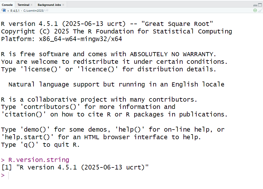
After installing both R and RStudio, double-click the RStudio icon to open it. In the console, type the following command:
R.version.string
Press Enter, and note down the displayed R version in your notebook.
To install Rtools
Download Rtools from here https://cran.r-project.org/bin/windows/Rtools/
Download the correct Rtools installer for your R version from the official Comprehensive R Archive Network (CRAN) page.
For example:
If your R version is 4.4.x, download Rtools44
If your R version is 4.3.x, download Rtools43
If your R version is 4.2.x, download Rtools42
If your R version is 4.0–4.1.x, download Rtools40
Steps
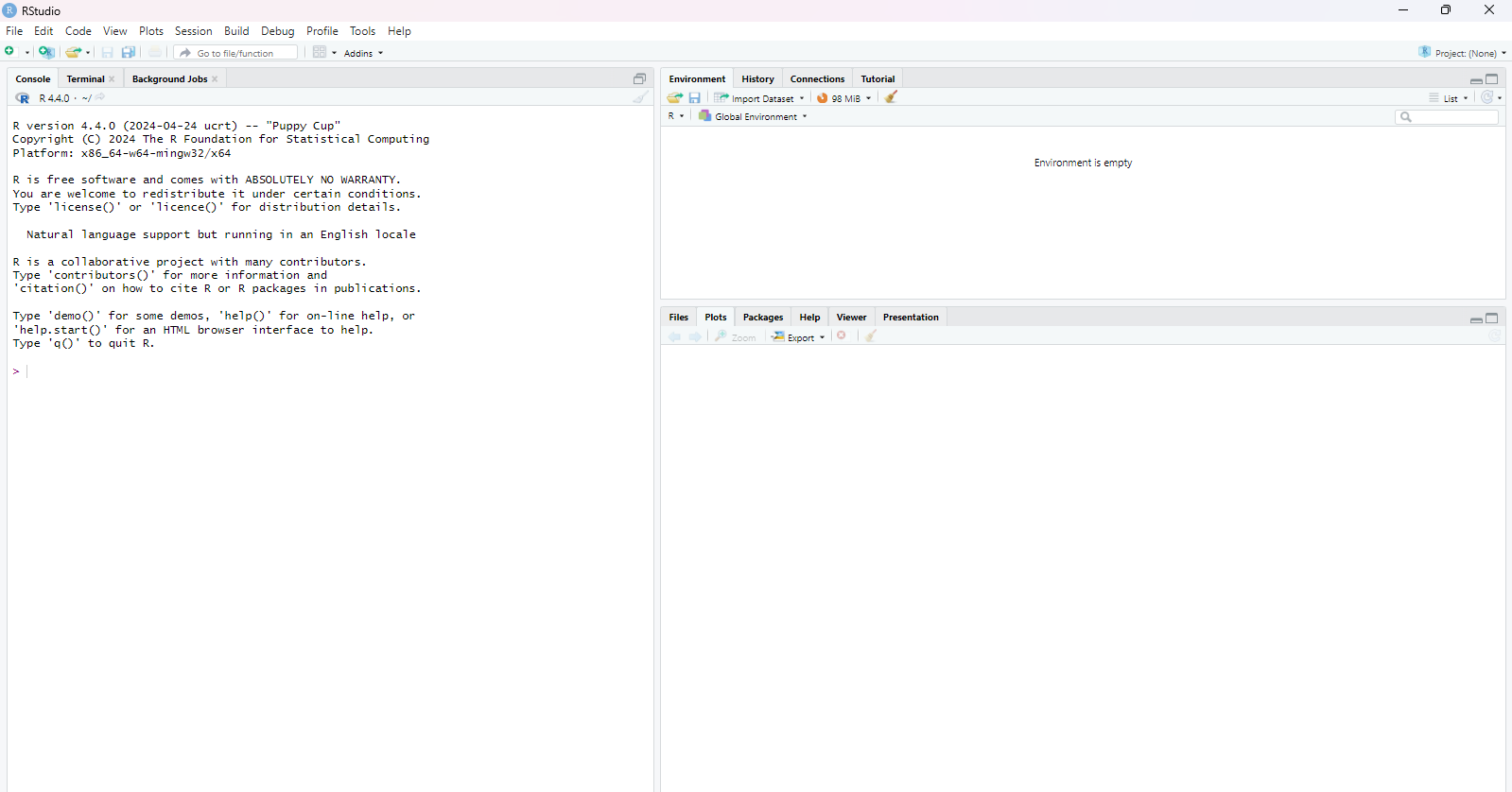 2. Go to File -> New File -> RScript
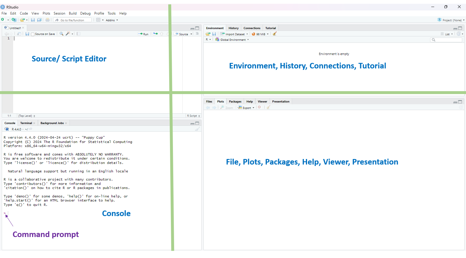
Source/Script: Where you write and save your R code.
Console: Where the code is executed and results are displayed.
Environment, History, Connections, Build, Tutorial: Where objects, past commands, database connections, projects, and learning aids are managed.
Files, Plots, Packages, Help, Viewer, Presentation: Where you browse files, view plots, manage packages, access help, preview outputs, and create presentations.
Creating an R Project means setting up a working directory where all your related files, such as scripts, data, and outputs are organized and stored together.
Steps:
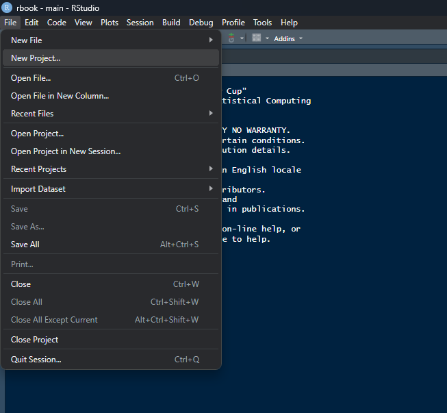
File -> New Project and follow the below steops
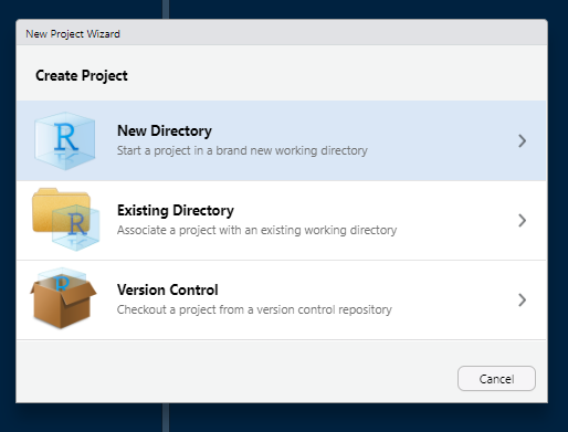
 Click on “New Directory”.
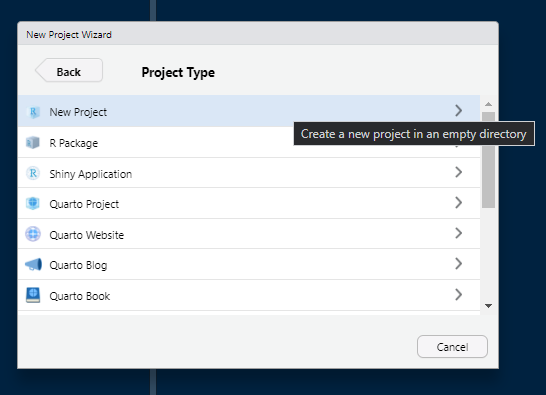
 Click on “New Project”.
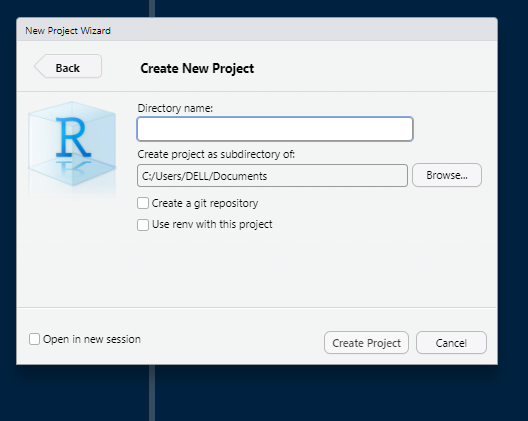
Give a project name and location to create project folder.
Once you have created a project, Windows users will see the project name displayed in the top-right corner of RStudio; for other operating systems, the location may vary but it will still be visible in the RStudio interface.
Type the following command on the console to view the project location.
getwd()This will give you the current working directory. The working directory is the folder where R reads and saves files. When you create an R Project, the project folder itself becomes the working directory, so the project and working directory are essentially the same.
Let’s type some simple commands. Type these in the console.
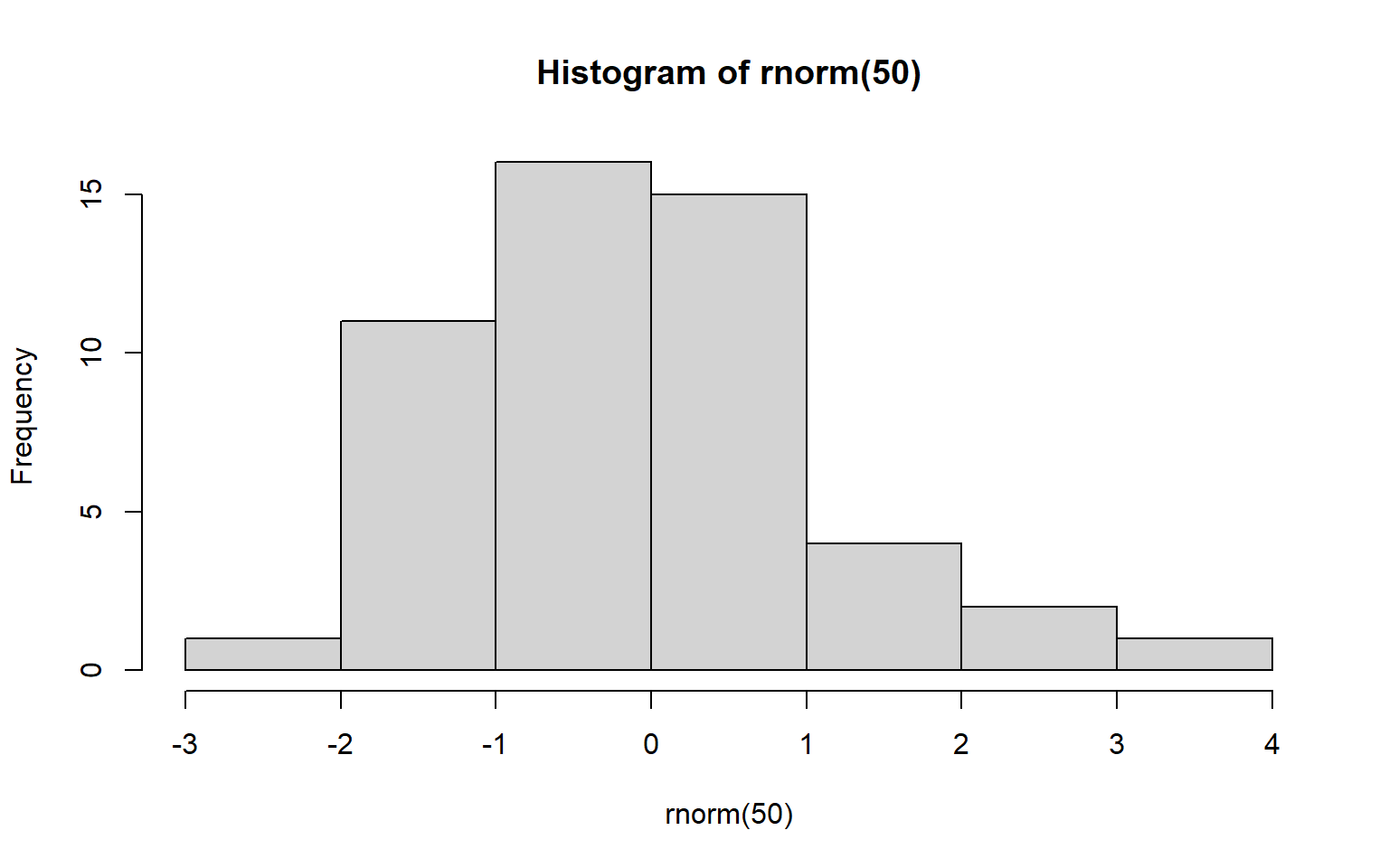
1 + 2[1] 31 * 100[1] 1001 / 100[1] 0.01rnorm(50) [1] 0.06521904 0.50754255 -0.06477693 -0.98669734 -1.42215540 -1.48852749
[7] -0.22637503 1.55099347 -0.58918021 -0.62523361 -0.01853335 1.28672051
[13] 1.42450806 -0.97262293 1.85150313 -0.08619909 0.01711273 2.35371891
[19] -1.09093500 0.53179014 0.77277099 -1.06019150 0.04141356 -2.08270872
[25] -0.22883505 0.34937099 -1.35541840 -1.77539082 -0.19191415 0.22090972
[31] -0.42502865 -0.22344388 0.82308138 0.71276526 -0.02787759 0.63547641
[37] -0.32422004 -0.02158706 1.38653711 0.31218900 0.41130577 -0.46838963
[43] -0.09707757 1.46380295 -0.68406538 -0.36138675 -0.28024751 -0.26112586
[49] 1.32779886 1.15915931In R, square brackets [ ] indicate the index or position of an element in a vector, list, or other data structure.
Commenting in R is adding notes or explanations in your code using #; comments are ignored when the code runs but help you and others understand the code.
Notice the changes in the “History” and “Environment” tabs.
A script file is a text file where you write and save R code so it can be run multiple times without retyping.
Open a script file and save it as “script1.R”. Type the following in the script file.
# 1. Assign values
x <- 10
y <- 5

# 2. Basic arithmetic
sum <- x + y
diff <- x - y
prod <- x * y
quot <- x / y

# 3. Create a vector
vec <- c(1, 2, 3, 4, 5)

# 4. Access elements (indexing)
vec[1]       # first element
vec[2:4]     # elements 2 to 4

# 5. Basic functions
mean(vec)    # mean of vector
sum(vec)     # sum of elements
length(vec)  # number of elements

# 6. Create a simple data frame
df <- data.frame(Name = c("A","B","C"), Score = c(10, 15, 20))

# 7. View data
df
head(df)     # first few rows

# 8. Help
?mean # get help for a functionA vector in R is a sequence of elements of the same type (numeric, character, or logical), and it is one of the basic data structures used to store and manipulate data.
# Create a numeric vector
numbers <- c(1, 2, 3, 4, 5)

# Create a character vector
fruits <- c("apple", "banana", "cherry", "apple")

# Access elements
numbers[1]      # first element
[1] 1fruits[2:3] # second and third elements[1] "banana" "cherry"# Basic operations
sum(numbers) # sum of all numbers[1] 15summary(numbers) # summary statistics Min. 1st Qu. Median Mean 3rd Qu. Max.
1 2 3 3 4 5 length(fruits) # number of elements[1] 4summary(fruits) # summary statistics Length Class Mode
4 character character table(fruits)fruits
apple banana cherry
2 1 1 Functions in R tell R to perform a specific task. To learn more about a function, type ?function_name in the console—this will open the function’s help file.
Example
?mean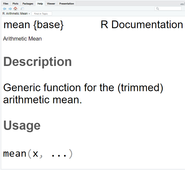
In the help file, mean {base} indicates that the mean function is part of the base package. You can think of packages in R like apps on your mobile phone: the default installation provides some basic packages, and for additional functionality, you can install extra packages just like installing new apps on your phone.
There are two ways that we can use to install packages.
Method 1
Go to the “Packages” tab and click install.
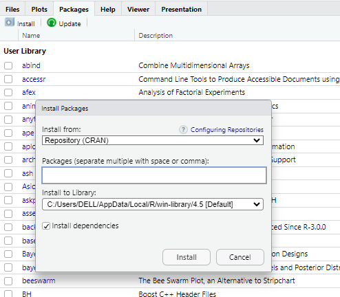
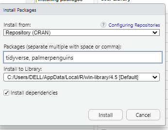
Then, type the names of the packages you need to install and click “install”.
The installation process will then start, and you will see progress messages displayed in the console.
Method 2
Type the following command on the console.
To install tidyverse package.
install.packages("tidyverse")To install palmerpenguins package.
install.packages("palmerpenguins")General format: Replace “xxx” with the name of the package you need to install.
install.packages(“xxx”)
To use a package in R, you first need to load it. Whenever you want to access a function from that package, use the following command.
For example to work with functions in tidyverse packages
TO work with palmerpenguins
A factor in R is used to represent categorical data. It stores both the values and the set of possible levels (categories) for the variable.
[1] Male   Female Female Male
Levels: Female Male
# Check the levels
levels(gender)[1] "Female" "Male" # Count occurrences of each level
table(gender)gender
Female   Male
2 2 summary(gender)Female Male
2 2 Your turn:
Create the gender vector as a character vector, then run table(gender) and summary(gender). Observe the differences in the outputs compared to when gender is a factor.
library(tibble)
ID <- 1:10
gender <- c(rep("male", 5), rep("female", 5))
height <- c(10, 20, 30, 14, 15, 21, 17, 12, 16, 23)
weight <- c(5, 10, 15, 7, 7.5, 10.5, 8.5, 6, 8, 11.5)
data <- tibble(ID=ID,
               Gender=gender,
               Weight=weight,
               Height=height)
data
# A tibble: 10 × 4
ID Gender Weight Height
<int> <chr> <dbl> <dbl>
1 1 male 5 10
2 2 male 10 20
3 3 male 15 30
4 4 male 7 14
5 5 male 7.5 15
6 6 female 10.5 21
7 7 female 8.5 17
8 8 female 6 12
9 9 female 8 16
10 10 female 11.5 23Some functions that we can use with tibbles
head(data)# A tibble: 6 × 4
ID Gender Weight Height
<int> <chr> <dbl> <dbl>
1 1 male 5 10
2 2 male 10 20
3 3 male 15 30
4 4 male 7 14
5 5 male 7.5 15
6 6 female 10.5 21tail(data)# A tibble: 6 × 4
ID Gender Weight Height
<int> <chr> <dbl> <dbl>
1 5 male 7.5 15
2 6 female 10.5 21
3 7 female 8.5 17
4 8 female 6 12
5 9 female 8 16
6 10 female 11.5 23glimpse(data)Rows: 10
Columns: 4
$ ID <int> 1, 2, 3, 4, 5, 6, 7, 8, 9, 10
$ Gender <chr> "male", "male", "male", "male", "male", "female", "female", "fe…
$ Weight <dbl> 5.0, 10.0, 15.0, 7.0, 7.5, 10.5, 8.5, 6.0, 8.0, 11.5
$ Height <dbl> 10, 20, 30, 14, 15, 21, 17, 12, 16, 23summary(data) ID Gender Weight Height
Min. : 1.00 Length:10 Min. : 5.000 Min. :10.00
1st Qu.: 3.25 Class :character 1st Qu.: 7.125 1st Qu.:14.25
Median : 5.50 Mode :character Median : 8.250 Median :16.50
Mean : 5.50 Mean : 8.900 Mean :17.80
3rd Qu.: 7.75 3rd Qu.:10.375 3rd Qu.:20.75
Max. :10.00 Max. :15.000 Max. :30.00 dim(data)[1] 10 4Convert gender into factor
data$Gender <- as_factor(data$Gender)
data
# A tibble: 10 × 4
ID Gender Weight Height
<int> <fct> <dbl> <dbl>
1 1 male 5 10
2 2 male 10 20
3 3 male 15 30
4 4 male 7 14
5 5 male 7.5 15
6 6 female 10.5 21
7 7 female 8.5 17
8 8 female 6 12
9 9 female 8 16
10 10 female 11.5 23glimpse(data)Rows: 10
Columns: 4
$ ID <int> 1, 2, 3, 4, 5, 6, 7, 8, 9, 10
$ Gender <fct> male, male, male, male, male, female, female, female, female, f…
$ Weight <dbl> 5.0, 10.0, 15.0, 7.0, 7.5, 10.5, 8.5, 6.0, 8.0, 11.5
$ Height <dbl> 10, 20, 30, 14, 15, 21, 17, 12, 16, 23summary(data) ID Gender Weight Height
Min. : 1.00 male :5 Min. : 5.000 Min. :10.00
1st Qu.: 3.25 female:5 1st Qu.: 7.125 1st Qu.:14.25
Median : 5.50 Median : 8.250 Median :16.50
Mean : 5.50 Mean : 8.900 Mean :17.80
3rd Qu.: 7.75 3rd Qu.:10.375 3rd Qu.:20.75
Max. :10.00 Max. :15.000 Max. :30.00 When you convert a charactor variable into factor you can see the counts.
Built-in datasets in R are preloaded or easily accessible datasets that come with R or its packages. They are mainly used for learning, practicing, and demonstrating data analysis techniques. You don’t need to import or download them. They are ready to use.
iris and penguins are two popular built-in-data sets in R
  Sepal.Length Sepal.Width Petal.Length Petal.Width Species
1          5.1         3.5          1.4         0.2  setosa
2          4.9         3.0          1.4         0.2  setosa
3          4.7         3.2          1.3         0.2  setosa
4          4.6         3.1          1.5         0.2  setosa
5          5.0         3.6          1.4         0.2  setosa
6 5.4 3.9 1.7 0.4 setosa# A tibble: 6 × 8
species island bill_length_mm bill_depth_mm flipper_length_mm body_mass_g
<fct> <fct> <dbl> <dbl> <int> <int>
1 Adelie Torgersen 39.1 18.7 181 3750
2 Adelie Torgersen 39.5 17.4 186 3800
3 Adelie Torgersen 40.3 18 195 3250
4 Adelie Torgersen NA NA NA NA
5 Adelie Torgersen 36.7 19.3 193 3450
6 Adelie Torgersen 39.3 20.6 190 3650
# ℹ 2 more variables: sex <fct>, year <int>To view all built-in-datasets, type
data() Pipe operator (|> or %>%) makes your codes more readable.
The following code
mean(1:10)[1] 5.5can be written as
1:10 |> mean()[1] 5.5If you are using ‘%>%’ pipe operator you need to install magrittr package in R.
Data manipulation is the process of changing, organizing, or summarizing data so it becomes easier to analyze, interpret, or visualize. We are going to learn 8 main data manipulation functions in the dplyr package.
library(palmerpenguins)
library(dplyr)
data("penguins")penguins# A tibble: 344 × 8
species island bill_length_mm bill_depth_mm flipper_length_mm body_mass_g
<fct> <fct> <dbl> <dbl> <int> <int>
1 Adelie Torgersen 39.1 18.7 181 3750
2 Adelie Torgersen 39.5 17.4 186 3800
3 Adelie Torgersen 40.3 18 195 3250
4 Adelie Torgersen NA NA NA NA
5 Adelie Torgersen 36.7 19.3 193 3450
6 Adelie Torgersen 39.3 20.6 190 3650
7 Adelie Torgersen 38.9 17.8 181 3625
8 Adelie Torgersen 39.2 19.6 195 4675
9 Adelie Torgersen 34.1 18.1 193 3475
10 Adelie Torgersen 42 20.2 190 4250
# ℹ 334 more rows
# ℹ 2 more variables: sex <fct>, year <int>colnames(penguins)[1] "species" "island" "bill_length_mm"
[4] "bill_depth_mm" "flipper_length_mm" "body_mass_g"
[7] "sex" "year" Type the following code to view the full data set.
View(penguins)penguins |>
filter(species == "Adelie", sex == "female")# A tibble: 73 × 8
species island bill_length_mm bill_depth_mm flipper_length_mm body_mass_g
<fct> <fct> <dbl> <dbl> <int> <int>
1 Adelie Torgersen 39.5 17.4 186 3800
2 Adelie Torgersen 40.3 18 195 3250
3 Adelie Torgersen 36.7 19.3 193 3450
4 Adelie Torgersen 38.9 17.8 181 3625
5 Adelie Torgersen 41.1 17.6 182 3200
6 Adelie Torgersen 36.6 17.8 185 3700
7 Adelie Torgersen 38.7 19 195 3450
8 Adelie Torgersen 34.4 18.4 184 3325
9 Adelie Biscoe 37.8 18.3 174 3400
10 Adelie Biscoe 35.9 19.2 189 3800
# ℹ 63 more rows
# ℹ 2 more variables: sex <fct>, year <int>Selects only female Adelie penguins.
penguins |>
  select(species, island, body_mass_g)
# A tibble: 344 × 3
species island body_mass_g
<fct> <fct> <int>
1 Adelie Torgersen 3750
2 Adelie Torgersen 3800
3 Adelie Torgersen 3250
4 Adelie Torgersen NA
5 Adelie Torgersen 3450
6 Adelie Torgersen 3650
7 Adelie Torgersen 3625
8 Adelie Torgersen 4675
9 Adelie Torgersen 3475
10 Adelie Torgersen 4250
# ℹ 334 more rows# A tibble: 344 × 8
species island bill_length_mm bill_depth_mm flipper_length_mm body_mass_g
<fct> <fct> <dbl> <dbl> <int> <int>
1 Gentoo Biscoe 49.2 15.2 221 6300
2 Gentoo Biscoe 59.6 17 230 6050
3 Gentoo Biscoe 51.1 16.3 220 6000
4 Gentoo Biscoe 48.8 16.2 222 6000
5 Gentoo Biscoe 45.2 16.4 223 5950
6 Gentoo Biscoe 49.8 15.9 229 5950
7 Gentoo Biscoe 48.4 14.6 213 5850
8 Gentoo Biscoe 49.3 15.7 217 5850
9 Gentoo Biscoe 55.1 16 230 5850
10 Gentoo Biscoe 49.5 16.2 229 5800
# ℹ 334 more rows
# ℹ 2 more variables: sex <fct>, year <int>penguins |>
arrange(body_mass_g)# A tibble: 344 × 8
species island bill_length_mm bill_depth_mm flipper_length_mm body_mass_g
<fct> <fct> <dbl> <dbl> <int> <int>
1 Chinstrap Dream 46.9 16.6 192 2700
2 Adelie Biscoe 36.5 16.6 181 2850
3 Adelie Biscoe 36.4 17.1 184 2850
4 Adelie Biscoe 34.5 18.1 187 2900
5 Adelie Dream 33.1 16.1 178 2900
6 Adelie Torgers… 38.6 17 188 2900
7 Chinstrap Dream 43.2 16.6 187 2900
8 Adelie Biscoe 37.9 18.6 193 2925
9 Adelie Dream 37.5 18.9 179 2975
10 Adelie Dream 37 16.9 185 3000
# ℹ 334 more rows
# ℹ 2 more variables: sex <fct>, year <int>penguins |>
mutate(body_mass_kg = body_mass_g / 1000)# A tibble: 344 × 9
species island bill_length_mm bill_depth_mm flipper_length_mm body_mass_g
<fct> <fct> <dbl> <dbl> <int> <int>
1 Adelie Torgersen 39.1 18.7 181 3750
2 Adelie Torgersen 39.5 17.4 186 3800
3 Adelie Torgersen 40.3 18 195 3250
4 Adelie Torgersen NA NA NA NA
5 Adelie Torgersen 36.7 19.3 193 3450
6 Adelie Torgersen 39.3 20.6 190 3650
7 Adelie Torgersen 38.9 17.8 181 3625
8 Adelie Torgersen 39.2 19.6 195 4675
9 Adelie Torgersen 34.1 18.1 193 3475
10 Adelie Torgersen 42 20.2 190 4250
# ℹ 334 more rows
# ℹ 3 more variables: sex <fct>, year <int>, body_mass_kg <dbl># A tibble: 1 × 1
mean_mass
<dbl>
1 4202.# A tibble: 3 × 2
species mean_mass
<fct> <dbl>
1 Adelie 3701.
2 Chinstrap 3733.
3 Gentoo 5076.penguins |>
rename(Mass_g = body_mass_g, Flipper_cm = flipper_length_mm)# A tibble: 344 × 8
species island bill_length_mm bill_depth_mm Flipper_cm Mass_g sex year
<fct> <fct> <dbl> <dbl> <int> <int> <fct> <int>
1 Adelie Torgersen 39.1 18.7 181 3750 male 2007
2 Adelie Torgersen 39.5 17.4 186 3800 female 2007
3 Adelie Torgersen 40.3 18 195 3250 female 2007
4 Adelie Torgersen NA NA NA NA <NA> 2007
5 Adelie Torgersen 36.7 19.3 193 3450 female 2007
6 Adelie Torgersen 39.3 20.6 190 3650 male 2007
7 Adelie Torgersen 38.9 17.8 181 3625 female 2007
8 Adelie Torgersen 39.2 19.6 195 4675 male 2007
9 Adelie Torgersen 34.1 18.1 193 3475 <NA> 2007
10 Adelie Torgersen 42 20.2 190 4250 <NA> 2007
# ℹ 334 more rowsif you want to keep the changes
penguins <- penguins |>
  rename(Mass_g = body_mass_g, Flipper_cm = flipper_length_mm)
penguins
# A tibble: 344 × 8
species island bill_length_mm bill_depth_mm Flipper_cm Mass_g sex year
<fct> <fct> <dbl> <dbl> <int> <int> <fct> <int>
1 Adelie Torgersen 39.1 18.7 181 3750 male 2007
2 Adelie Torgersen 39.5 17.4 186 3800 female 2007
3 Adelie Torgersen 40.3 18 195 3250 female 2007
4 Adelie Torgersen NA NA NA NA <NA> 2007
5 Adelie Torgersen 36.7 19.3 193 3450 female 2007
6 Adelie Torgersen 39.3 20.6 190 3650 male 2007
7 Adelie Torgersen 38.9 17.8 181 3625 female 2007
8 Adelie Torgersen 39.2 19.6 195 4675 male 2007
9 Adelie Torgersen 34.1 18.1 193 3475 <NA> 2007
10 Adelie Torgersen 42 20.2 190 4250 <NA> 2007
# ℹ 334 more rowspenguins |>
slice(5:10)# A tibble: 6 × 8
species island bill_length_mm bill_depth_mm Flipper_cm Mass_g sex year
<fct> <fct> <dbl> <dbl> <int> <int> <fct> <int>
1 Adelie Torgersen 36.7 19.3 193 3450 female 2007
2 Adelie Torgersen 39.3 20.6 190 3650 male 2007
3 Adelie Torgersen 38.9 17.8 181 3625 female 2007
4 Adelie Torgersen 39.2 19.6 195 4675 male 2007
5 Adelie Torgersen 34.1 18.1 193 3475 <NA> 2007
6 Adelie Torgersen 42 20.2 190 4250 <NA> 2007