6 Probability and Distribution Theory

6.1 What is Probability?

Probability is a quantitative measure of uncertainty.
A number that conveys the strength of our belief in the occurrence of an uncertain event.

6.2 Terminology

Experiment

Statisticians use the word experiment to describe any process that generates a set of data. This involves observing or counting or measuring.

Random Experiment

All possible outcomes can be specified in advance.
It can be repeated in an identical fashion.
The same outcome may not occur on various repetitions so that the actual outcome is not known in advance.

Outcomes

The results one obtains from an experiment

Sample space

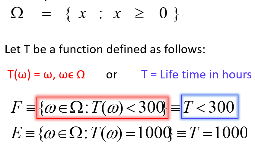
The set of all possible outcomes of an experiment.

Events

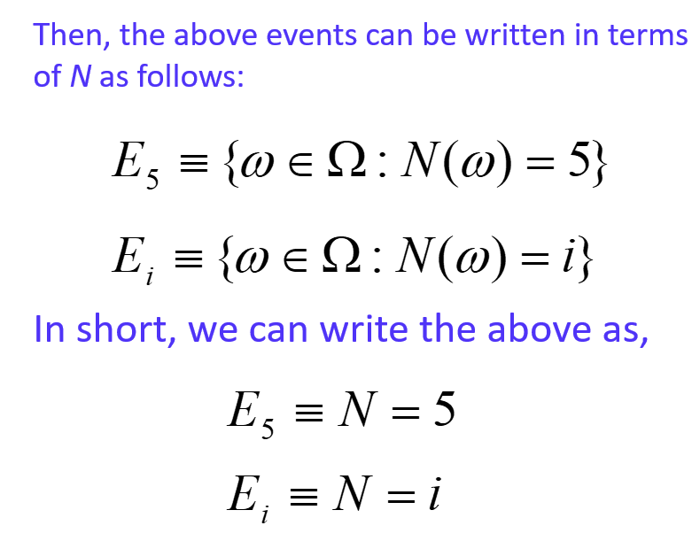
An event is a subset of the set of all possible results of some action or a process or a procedure.
Events are usually denoted by capital English letters A, B, C, D, E etc.
Events are of two types,
- Simple event: An event containing only one outcome
- Compound event: An event containing more than one outcome

Random Variable

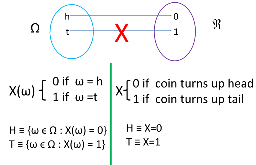
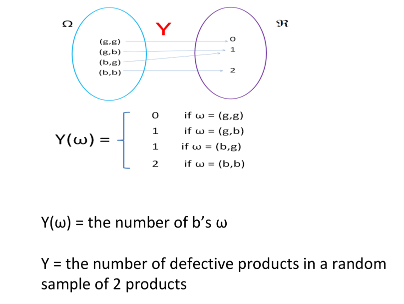
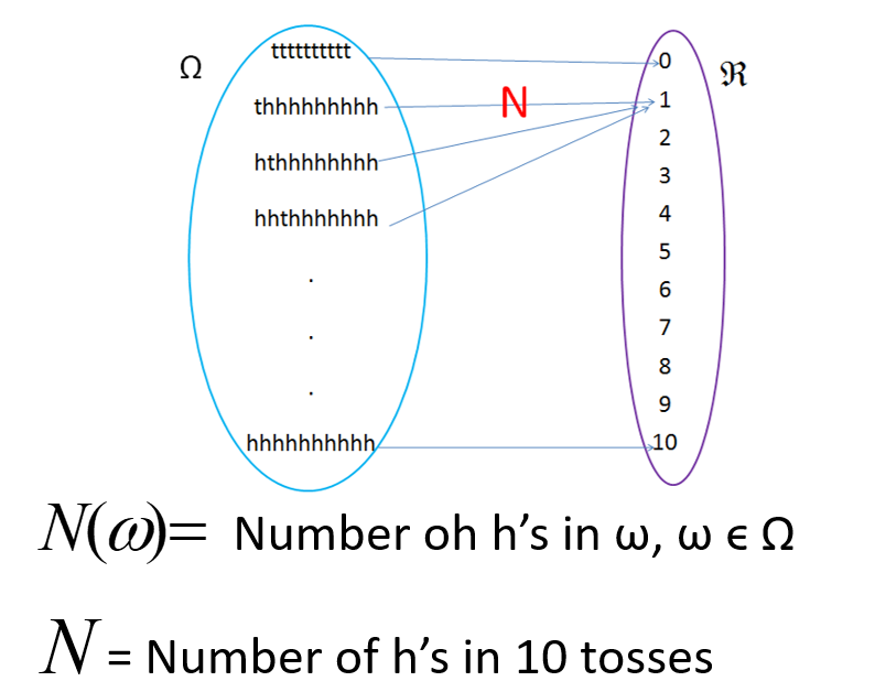
Let \Omega be a sample space. Let X be a function from \Omega to \mathbb{R} (i.e., X: \Omega \to \mathbb{R}). Then X is called a random variable.

Random variables are denoted by capital English letters.

Event 1

Event 2

Event 3

Event 4

6.3 Event Operations

Intersection
Union
Complement

6.4 Axioms of probability

Axiom 1: For any event A, P (A) ≥ 0

Axiom 2: P(\Omega) = 1

Axiom 3:

If A_1, A_2, \dots, A_k is a finite collection of mutually exclusive events, then P(A_1 \cup A_2 \cup \dots \cup A_k) = P(A_1) + P(A_2) + \dots + P(A_k) = \sum_{i=1}^{k} P(A_i).
If A_1, A_2, \dots is an infinite collection of mutually exclusive events, then P\Big(\bigcup_{i=1}^{\infty} A_i \Big) = \sum_{i=1}^{\infty} P(A_i).

Axioms 1 and 2 imply that for any event E, 0 \leq P(E) \leq 1.

The probability of an impossible event is 0.

The probability of an event that is certain to occur is 1.

6.5 Interpretation of probability

Relative frequency interpretation.

The probability of an event E related to a random experiment can be interpreted as the ’approximate proportion of times that E occurs if we repeat the experiment very large number of times.

Example: A wildlife biologist could then say that the probability that a randomly selected turtle from this population has the disease is 0.05. This means, if we observe a very large population of sea turtles in a certain coastal region, the proportion of turtles carrying a particular shell disease might be approximately 5%.

Subjective interpretation.

Example: A marine biologist feels that there is a 60% chance that a rescued dolphin will successfully reintegrate into the wild, based on her past experience with similar rescues and her knowledge of the dolphin’s behavior.

6.6 Methods for Determining Probability

Classical method
Relative frequency method
Subjective method
Using probability models

6.7 Classical Method

Probability is calculated based on the sample space.
No need to carry out any experiment. It is enough to know the sample space.
This approach can be used only if,
- the sample space consists of finite number of outcomes.
- all the outcomes are ‘equally likely’

Then, the probability of event E is given by,

P(E) = \frac{n(E)}{n(\Omega)}

6.8 Exercise

Q1: What is the probability of obtaining ‘Head’ in a single toss of an unbiased coin?

Q2: Two fair dice are tossed. Find the probability that sum of the dice equals seven.

Q3: A box contains 3 white balls and 2 black balls. Two balls are taken one after the other without replacement. Write down the sample space. Find the probability of getting one white ball and one black ball.

\Omega = \{(W,W), (W,B), (B,W), (B,B)\}

Are the outcomes of this sample space equally likely?

Can you write the sample space so that outcomes will be equally likely?

6.9 Relative frequency method (Empirical probability)

P(E) =\frac{\text{number of times E occurred}}{\text{number of times trial was repeated}} ## Exercise

Q1: A wildlife researcher observes 500 frogs in a wetland and records that 75 of them have a certain skin fungus.

Using the relative frequency approach, estimate the probability that a randomly selected frog from this wetland has the skin fungus.

Q2: During a bird migration study, a biologist counts 800 birds and finds that 160 of them are male sparrows.

Using the relative frequency approach, what is the probability that a randomly selected bird from this group is a male sparrow?

6.10 Subjective Method

Usually based on an educated guess or estimate, employing opinions and inexact information.

6.11 Conditional Probability

The conditional probability of an event A given that event B has occurred is denoted by P(A \mid B) and is defined as:

P(A \mid B) = \frac{P(A \cap B)}{P(B)}, \quad \text{for } P(B) > 0

6.12 Multiplication Rule

Rearranging the formula of conditional probability, we get the :

P(A \cap B) = P(A \mid B) \cdot P(B)

6.13 Extension for multiple events

For three events A, B, and C, the multiplication rule can be extended as:

P(A \cap B \cap C) = P(A) \cdot P(B \mid A) \cdot P(C \mid A \cap B)

6.14 Mutually Exclusive Events

Two or more events are mutually exclusive if they cannot occur at the same time.

P(A \cap B) = 0

Example (Zoology):
In a bird survey, observing a bird as either a sparrow or an eagle in a single sighting is mutually exclusive — the bird cannot be both at the same time.

6.15 Exhaustive Events

A set of events is exhaustive if at least one of them must occur, meaning they cover all possible outcomes.

P(A_1 \cup A_2 \cup \dots \cup A_n) = 1

Example (Zoology):
Observing a frog in a wetland, it must either be male or female. These categories are exhaustive because they cover all possible frogs.

6.16 Independent Events

Two events A and B are independent if the occurrence of one does not affect the probability of the other.

P(A \cap B) = P(A) \cdot P(B)

Example (Zoology):
The event that a sea turtle lays eggs today and the event that a crab crosses the beach are independent — one does not affect the other.

6.17 Combinations of Events: Mutual Exclusivity and Exhaustiveness

In-class

6.18 Rules of Probability

1. Complement Rule

The probability of the complement of an event A, denoted by A^c, is:

P(A^c) = 1 - P(A)

2. Addition Rule

For any two events A and B:

P(A \cup B) = P(A) + P(B) - P(A \cap B)

For mutually exclusive events A and B:

P(A \cup B) = P(A) + P(B)

3. Multiplication Rule

Conditional probability:

P(A \mid B) = \frac{P(A \cap B)}{P(B)}, \quad P(B) > 0

Multiplication rule:

P(A \cap B) = P(A \mid B) \cdot P(B)

Extension to multiple events A_1, A_2, \dots, A_n:

P(A_1 \cap A_2 \cap \dots \cap A_n) = P(A_1) \cdot P(A_2 \mid A_1) \cdot \dots \cdot P(A_n \mid A_1 \cap \dots \cap A_{n-1})

6.19 4. Law of Total Probability

If \{B_1, B_2, \dots, B_n\} is a partition of the sample space \Omega, then for any event A:

P(A) = \sum_{i=1}^{n} P(A \mid B_i) \cdot P(B_i)

6.20 5. Bayes’ Theorem

For events A and B_i with P(B_i) > 0:

P(B_i \mid A) = \frac{P(A \mid B_i) \cdot P(B_i)}{\sum_{j=1}^{n} P(A \mid B_j) \cdot P(B_j)}

6.21 Exercise

Question 1

A wildlife researcher studies frogs in three ponds: Pond A, Pond B, and Pond C.

Pond A has 50 frogs, Pond B has 30 frogs, and Pond C has 20 frogs.

The probability that a frog in Pond A is infected with a skin fungus is 0.1, in Pond B is 0.2, and in Pond C is 0.3.

If a frog is randomly selected from all ponds, what is the probability that it is infected?
Suppose a randomly selected frog is found to be infected. What is the probability that it came from Pond B?

Question 2

A wildlife biologist tests a population of 1000 bats for a viral infection using a diagnostic test.

200 bats are actually infected.

The test correctly identifies 180 of the infected bats as positive.

Among the 800 uninfected bats, the test correctly identifies 720 as negative.

Tasks:

Calculate the sensitivity of the test.

Calculate the specificity of the test.

6.22 Probability Distributions

Below are four commonly used distributions in zoological studies.

Binomial Distribution

The Binomial distribution models the number of successes in a fixed number of independent trials, where each trial has two outcomes (success/failure).

Let X be the number of frogs infected out of 10 observed.

P(X = x) = \binom{n}{x} p^x (1 - p)^{n - x}

where
- n = number of trials (e.g., number of frogs observed)
- p = probability of success (e.g., infection)
- x = number of successes (e.g., frogs infected)

Example:
A wildlife biologist observes 10 frogs and records whether each frog is infected with a fungus (infected = success).

If the probability of infection is 0.2, the number of infected frogs follows a Binomial distribution.

What is the probability that exactly 3 frogs are infected?

Calculation:

P(X = 3) = \binom{10}{3} 0.2^3 (1 - 0.2)^{10 - 2}

R Code:

# Parameters
n <- 10    # number of frogs
p <- 0.2   # probability of infection

# Probability of exactly 3 infected frogs
dbinom(3, size = n, prob = p)

[1] 0.2013266

Poisson Distribution

The Poisson distribution describes the number of events that occur in a fixed time or space interval when events happen independently and at a constant average rate.

P(X = x) = \frac{e^{-\lambda} \lambda^x}{x!}

where:
- \lambda: average number of events per interval
- x: number of observed events

Example

A field researcher records bird calls in a forest.
On average, there are ( = 5 ) calls per minute.

What is the probability that exactly 3 bird calls are heard in one minute?

Let X be the number of bird calls within a minute.

P(X = 3) = \frac{e^{-5} 5^3}{3!} = 0.1404

Therefore, the probability of hearing exactly 3 calls in one minute is 0.1404.

R Code:

lambda <- 5
dpois(3, lambda)

[1] 0.1403739

What is the probability that exactly 3 bird calls are heard in one hour?

Let X be the number of bird calls heard in one hour.

Then the average number of bird calls per minute is 60 \times 5 = 300.

lambda_hour <- 5 * 60  # 300 bird calls per hour
x <- 3

# Probability of exactly 3 bird calls in an hour
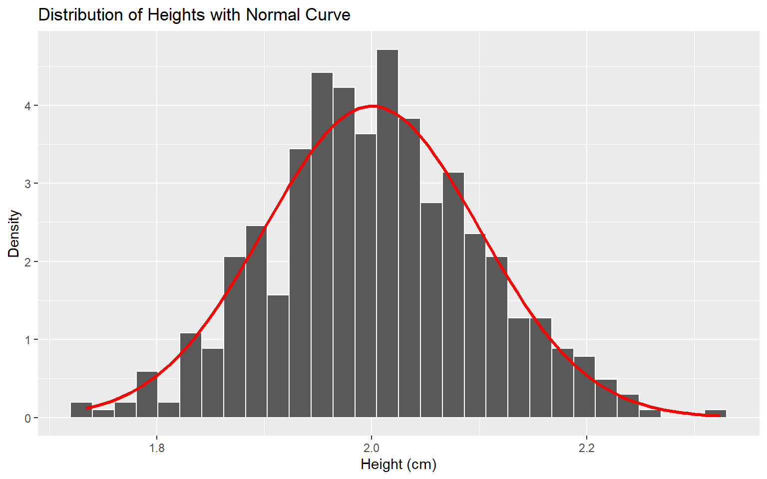
dpois(x, lambda_hour)

[1] 2.31669e-124

Normal Distribution

The Normal distribution is used to describe continuous measurements such as body length, weight, or temperature that cluster around a mean value.

f_X(x) = \frac{1}{\sqrt{2 \pi \sigma^2}} \, e^{ - \frac{(x - \mu)^2}{2 \sigma^2} }

Where:
- x = observed value
- \mu = mean of the distribution
- \sigma = standard deviation
- f_X(x) = probability density at x

Illustration

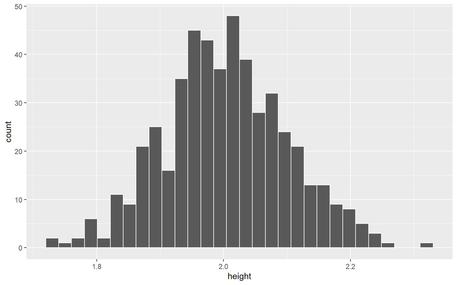
Height of 500 elephants.

  [1] 1.9 2.0 2.2 2.0 2.0 2.2 2.0 1.9 1.9 2.0 2.1 2.0 2.0 2.0 1.9 2.2 2.0 1.8
 [19] 2.1 2.0 1.9 2.0 1.9 1.9 1.9 1.8 2.1 2.0 1.9 2.1 2.0 2.0 2.1 2.1 2.1 2.1
 [37] 2.1 2.0 2.0 2.0 1.9 2.0 1.9 2.2 2.1 1.9 2.0 2.0 2.1 2.0 2.0 2.0 2.0 2.1
 [55] 2.0 2.2 1.8 2.1 2.0 2.0 2.0 1.9 2.0 1.9 1.9 2.0 2.0 2.0 2.1 2.2 2.0 1.8
 [73] 2.1 1.9 1.9 2.1 2.0 1.9 2.0 2.0 2.0 2.0 2.0 2.1 2.0 2.0 2.1 2.0 2.0 2.1
 [91] 2.1 2.1 2.0 1.9 2.1 1.9 2.2 2.2 2.0 1.9 1.9 2.0 2.0 2.0 1.9 2.0 1.9 1.8
[109] 2.0 2.1 1.9 2.1 1.8 2.0 2.1 2.0 2.0 1.9 1.9 1.9 2.0 1.9 2.0 2.0 2.2 1.9
[127] 2.0 2.0 1.9 2.0 2.1 2.0 2.0 2.0 1.8 2.1 1.9 2.1 2.2 1.9 2.1 2.0 1.8 1.8
[145] 1.8 1.9 1.9 2.1 2.2 1.9 2.1 2.1 2.0 1.9 2.0 2.0 2.1 2.0 2.1 2.0 2.1 1.9
[163] 1.9 2.3 2.0 2.0 2.1 2.0 2.1 2.0 2.0 2.0 2.0 2.2 1.9 1.9 2.0 2.0 2.0 2.0
[181] 1.9 2.1 2.0 1.9 2.0 2.0 2.1 2.0 2.1 2.0 2.0 2.0 2.0 1.9 1.9 2.2 2.1 1.9
[199] 1.9 1.9 2.2 2.1 2.0 2.1 2.0 2.0 1.9 1.9 2.2 2.0 2.0 2.0 2.1 1.9 1.9 2.2
[217] 2.0 1.9 1.9 1.9 1.9 2.1 2.1 2.1 2.0 2.0 1.9 1.9 2.1 1.9 2.2 2.0 2.0 1.9
[235] 1.9 1.9 2.0 2.0 2.0 1.9 1.9 1.9 2.1 1.9 2.0 2.2 2.0 1.9 1.9 2.0 2.0 1.9
[253] 2.0 2.0 2.2 2.0 2.1 2.1 2.0 1.8 1.9 2.0 2.0 2.1 2.2 2.2 2.0 1.8 2.0 2.0
[271] 2.1 2.1 2.1 1.9 2.1 2.0 2.0 2.0 2.0 2.0 1.8 2.1 2.0 2.0 2.0 2.0 2.0 2.2
[289] 2.0 2.0 2.1 2.1 2.1 1.9 2.2 2.0 2.2 1.9 2.0 2.1 1.9 1.9 1.9 1.9 2.0 2.0
[307] 1.8 2.0 2.1 2.2 2.1 2.1 1.8 1.9 2.0 2.1 2.0 1.9 2.2 2.1 2.0 2.1 1.9 2.1
[325] 1.9 2.1 2.0 2.1 2.1 2.0 2.1 1.9 1.9 2.2 2.0 1.8 1.9 2.0 2.1 2.0 2.1 2.1
[343] 2.2 2.0 2.0 1.8 2.0 1.9 1.9 2.0 2.1 1.8 2.0 2.0 1.9 2.0 2.0 2.0 1.8 2.3
[361] 2.0 2.1 2.0 2.1 2.1 2.0 2.0 1.9 2.1 2.0 2.2 1.8 2.0 2.1 2.1 1.9 1.9 2.0
[379] 2.0 1.8 2.0 2.0 2.0 1.9 2.0 2.1 2.0 1.9 2.0 2.0 1.9 1.8 2.1 1.9 1.9 2.2
[397] 1.9 2.1 1.9 2.0 2.0 1.9 1.9 2.0 2.1 1.8 2.0 2.1 1.9 2.0 2.0 2.0 2.1 2.0
[415] 2.0 1.7 2.0 2.0 2.1 1.9 2.2 2.0 2.0 2.1 1.9 2.0 2.2 2.0 2.2 1.9 2.0 2.0
[433] 2.0 1.9 2.0 1.9 2.1 2.1 1.8 2.1 1.9 2.0 2.1 2.0 1.9 2.0 2.0 2.1 1.8 1.8
[451] 2.1 2.1 2.0 2.1 2.1 1.7 2.1 2.0 2.0 2.0 2.1 2.0 2.1 2.0 1.9 2.1 2.1 2.2
[469] 2.0 2.1 2.2 2.0 1.9 2.0 2.0 2.0 2.2 2.0 2.0 2.0 2.0 2.0 2.1 2.0 2.1 2.1
[487] 2.1 1.9 2.2 2.0 2.0 2.1 2.1 1.9 1.9 1.9 2.0 2.0 2.0 2.1

Distribution of height

Approximate the shape of the distribution using normal distribution density

Example

Suppose the body weights of adult lizards in a population are normally distributed with:

\mu = 150 \text{ g}, \quad \sigma = 20 \text{ g}

Define the random variable:

X = \text{body weight of a randomly selected lizard (g)}

What is the probability that a randomly selected lizard weighs less than 130 g?

We standardize using the z-score formula:

Z = \frac{X - \mu}{\sigma} = \frac{130 - 150}{20} = -1

Using the cumulative distribution function (CDF):

P(X < 130) = P(Z < -1) = 0.1587

R code:

Method 1

# Parameters
mean_weight <- 150
sd_weight <- 20

# Probability of weight less than 130 g
pnorm(130, mean = mean_weight, sd = sd_weight)

[1] 0.1586553

Method 2:

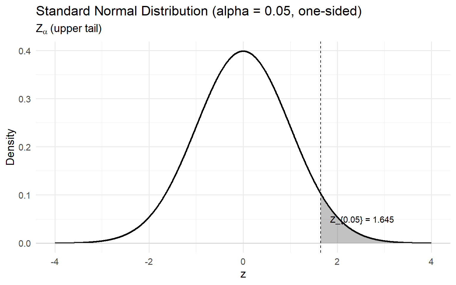
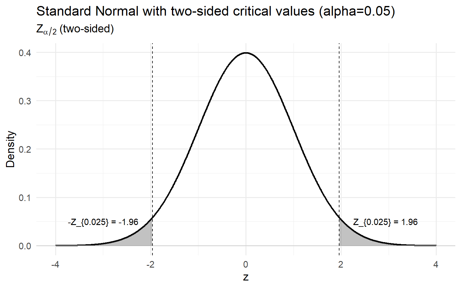
[1] 0.1586553

Illustrating the idea of Z_{\alpha} notation

The notation Z_{\alpha} represents the critical value of the standard normal distribution (mean = 0, standard deviation = 1) that leaves an upper-tail area of \alpha. It is commonly used in hypothesis testing to mark the boundary of the rejection region at a significance level \alpha.

P(Z > Z_{\alpha}) = \alpha, \quad \text{where } Z \sim N(0,1)

For example, when the significance level is \alpha = 0.05,

Z_{0.05} = 1.645

This means that 5% of the standard normal distribution lies to the right of 1.645.

In hypothesis testing:

For a one-sided test, the rejection region is Z > Z_{\alpha} (upper tail) or Z < -Z_{\alpha} (lower tail).
For a two-sided test, the critical values are \pm Z_{\alpha/2}, leaving \alpha/2 area in each tail.

Graphically, Z_{\alpha} appears as a vertical line on the standard normal curve, with the shaded region beyond it representing the probability \alpha.

R Code

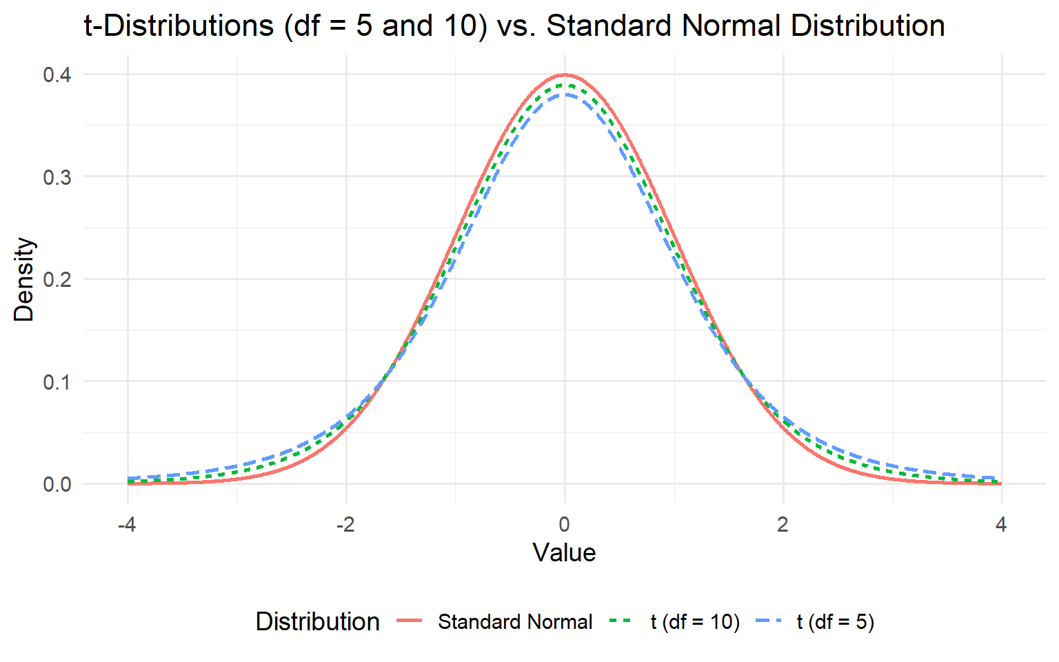
qnorm(0.05)

[1] -1.644854

qnorm(0.5)

[1] 0

6.23 t-distribution

The t-distribution is similar to the standard normal distribution but has heavier tails, especially for small sample sizes.

t_{df} \xrightarrow[df \to \infty]{} N(0,1)

R Code

pt(0, df=10)

[1] 0.5

pt(5, df=10)

[1] 0.9997313

qt(0.2, df=10)

[1] -0.8790578