worldbankdata |>
  ggplot(aes(x = Electricity)) +   geom_density()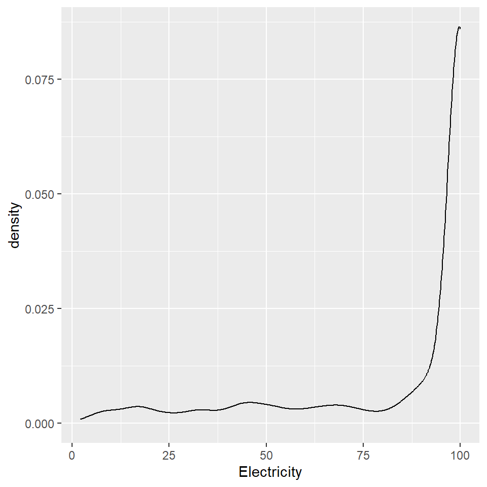
Package
ggplot2 (Wickham 2016)
Description
Computes and draws kernel density estimation.
Understandable aesthetics
required aesthetics
x, y
optional aesthetics
alpha, colour, fill, group, linetype, linewidth, weight
See also
Example
worldbankdata |>
ggplot(aes(x = Electricity)) + geom_density()
Package
ggridges (Wilke 2023)
Description
Draws a density plot same as geom_density. The difference is that the geom draws a ridgeline (line with filled area underneath).
Understandable aesthetics
required aesthetics
x
y
optional aesthetics
alpha, colour, fill, group, linetype, linewidth, weight
See also
Example
library(ggridges)
worldbankdata |>
  ggplot(aes(x = Electricity)) +
  geom_density_line()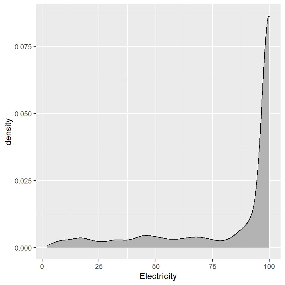
Package
ggplot2 (Wickham 2016)
Description
Computes a 2D kernel density estimation using MASS::kde2d() and display the results with contours.
Understandable aesthetics
stat_density
required aesthetics
x
y
optional aesthetics
alpha, colour, group, linetype, linewidth
See also
Example
a1 <- worldbankdata |>
  ggplot(aes(y = Cooking, x=Electricity)) +
  geom_density_2d() +
  xlim(0, 100) +
  ylim(0, 100) +
  theme(aspect.ratio = 1) +
  labs(title = "a1: geom_density_2d only")
a2 <- worldbankdata |>
  ggplot(aes(y = Cooking, x=Electricity)) +
  geom_point() +
  geom_density_2d() +
  theme(aspect.ratio = 1) +
  labs(title = "a2: geom_point and \n geom_density_2d")

a1|a2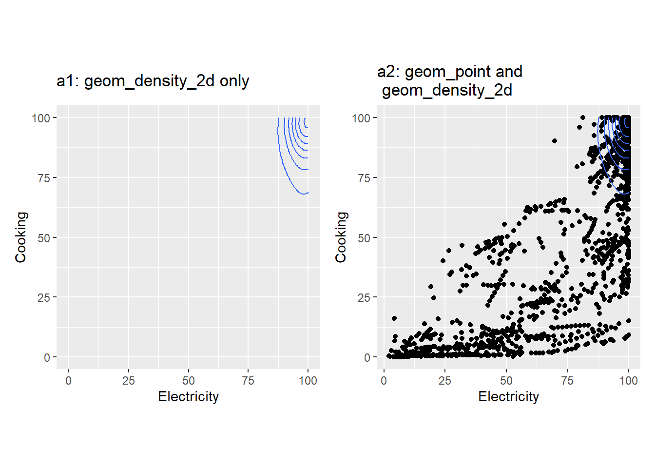
Package
ggplot2 (Wickham 2016)
Description
Computes a 2D kernel density estimation using MASS::kde2d() and display the results with filled contour bands.
Understandable aesthetics
required aesthetics
x
y
optional aesthetics
alpha, colour, group, linetype, linewidth, subgroup
See also
Example
a1 <- worldbankdata |>
  filter(Year == "2021") |>
  ggplot(aes(y = Cooking, x=Electricity)) +
  geom_density_2d_filled() +
  labs(title = "a1: geom_density_2d_filled only") +
  theme( aspect.ratio = 1)
a2 <- worldbankdata |>
  filter(Year == "2020") |>
  ggplot(aes(y = Cooking, x=Electricity)) +
  geom_density_2d_filled(alpha = 0.5) +
    geom_point() +
  labs(title = "a2: geom_point and \n geom_density_2d_filled") +
  theme( aspect.ratio = 1)
a3 <- worldbankdata |>
  filter(Year == "2020") |>
  ggplot(aes(y = Cooking, x=Electricity)) +
  geom_point(alpha=0.5) +
  labs(title = "a3: geom_point") +
  theme(aspect.ratio = 1)
a1 / a2 / a3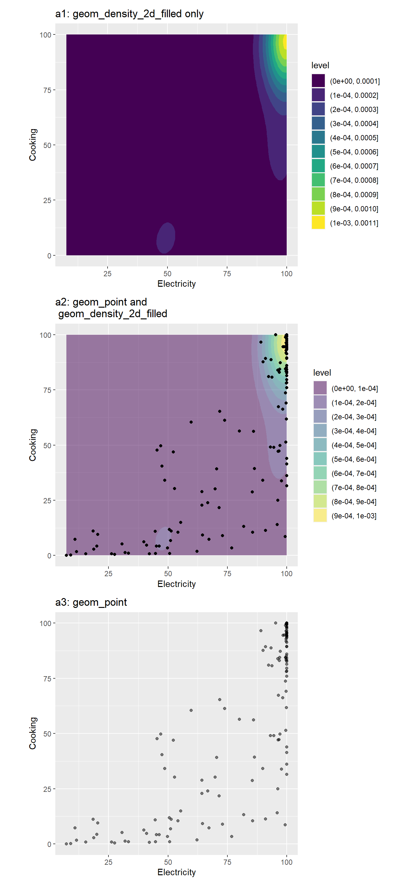
Package
ggridges (Wilke 2023)
Description
Arranges multiple density plots in a staggered fashion.
Understandable aesthetics
required aesthetics
x, y
optional aesthetics
colour, fill, group, height, alpha, linetype, linewidth, scale, rel_min_height
See also
Example
library(ggridges)
 worldbankdata |>
  ggplot(aes(y = Income, x=Electricity)) +
geom_density_ridges() 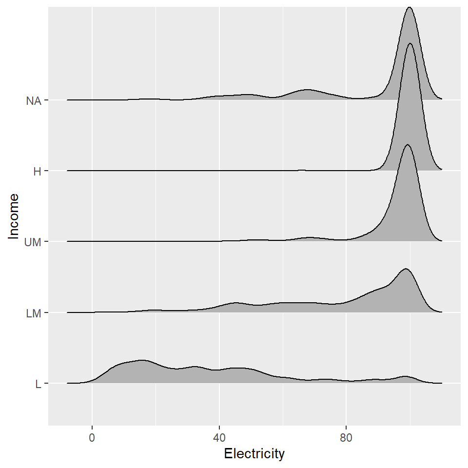
Package
ggridges (Wilke 2023)
Description
Arranges multiple density plots in a staggered fashion.
Understandable aesthetics
required aesthetics
x, y
optional aesthetics
colour, fill, group, height, alpha, linetype, linewidth, scale, rel_min_height
See also
Example
library(ggridges)
 worldbankdata |>
  ggplot(aes(y = Income, x=Electricity, fill=stat(x))) +
  geom_density_ridges_gradient() +
  scale_fill_viridis_c()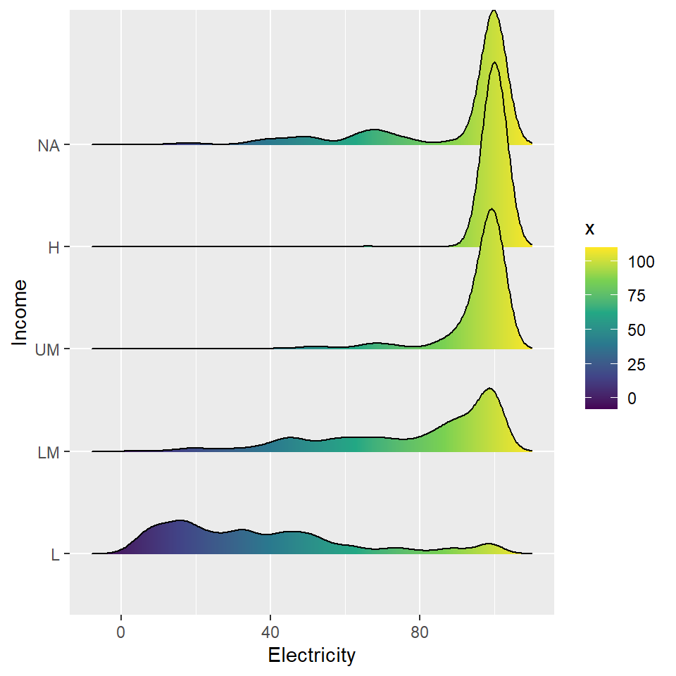
Package
directlabels (Hocking 2023)
Description
Display direct labels on the plot.
Understandable aesthetics
layer
See also
Example
library(directlabels)
a1 <- worldbankdata |>
  ggplot(aes(y = Cooking, x=Electricity)) +
  geom_point(aes(col=Income)) +
  theme(aspect.ratio = 1) +
  scale_color_brewer(palette = "Set1")
a1 +
  geom_dl(aes(label=Income), method="smart.grid")+
  scale_shape_manual(values=c(H = 1,
                              UM = 6,
                              L = 3,
                              LM = 2),
                     guide="none")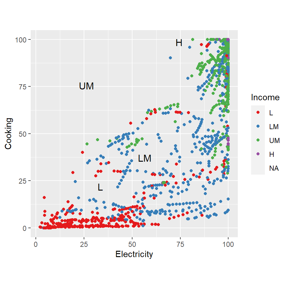
Package
ggplot2 (Wickham 2016)
Description
Create dotplot.
required aesthetics
x or y
optional aesthetics
alpha, colour, fill , group, linetype, stroke
See also
Example
worldbankdata |>
  ggplot(aes(x=Cooking)) +
  geom_dotplot(binwidth = 1) +
  theme(legend.position="none", aspect.ratio = 1)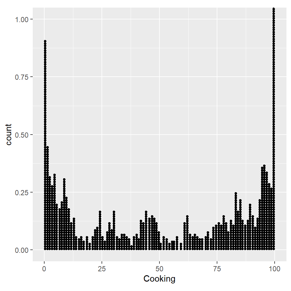
Package
ggforce (Pedersen 2022)
Description
Display voronoi tesselation and delaunay triangulation.
Understandable aesthetics
required aesthetics
x or y
optional aesthetics
alpha, colour, fill , linetype, size
See also
Example
library(ggforce)
library(deldir) #to calculate delaunay triangulation
a1 <- worldbankdata |>
  filter(Income == "L") |>
  ggplot(aes(x=Cooking, y=Electricity)) +
  geom_delaunay_tile(alpha=0.5) +
  labs(title = "a1: geom_delaunay_tile only") +
  theme(aspect.ratio = 1)

a2 <- worldbankdata |>
  filter(Income == "L") |>
  ggplot(aes(x=Cooking, y=Electricity)) +
  geom_point() +
  geom_delaunay_tile(alpha=0.5) +
  labs(title = "a2: geom_point and \n geom_delaunay_tile") +
  theme(aspect.ratio = 1)
a1 | a2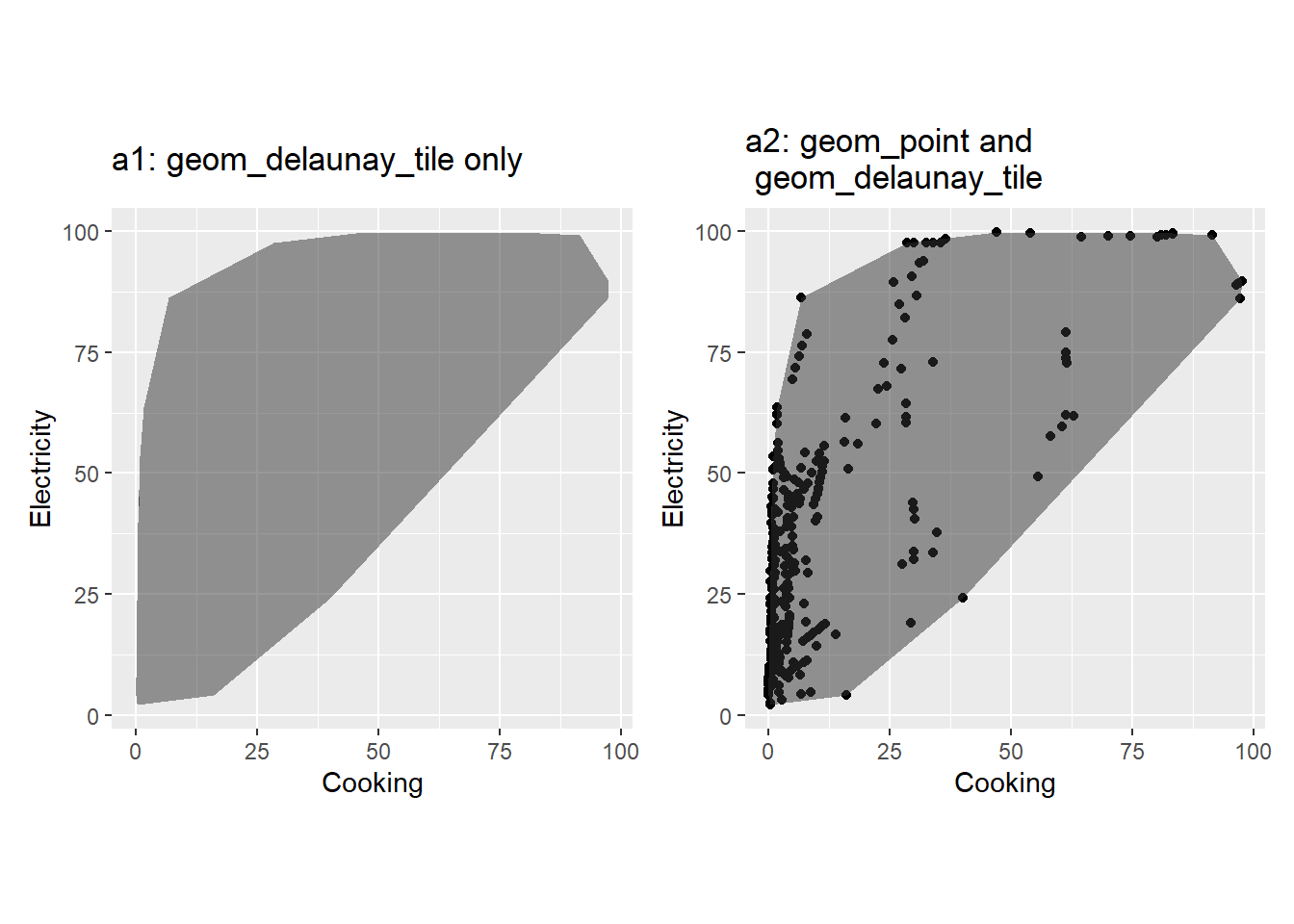
Package
ggforce (Pedersen 2022)
Description
Display voronoi tesselation and delaunay triangulation.
Understandable aesthetics
required aesthetics
x or y
optional aesthetics
alpha, colour, fill , linetype, size
See also
Example
library(ggforce)
library(deldir) #to calculate delaunay triangulation

a1 <- worldbankdata |>
  filter(Income == "L") |>
  ggplot(aes(x=Cooking, y=Electricity)) +
  geom_delaunay_segment() +
  theme(aspect.ratio = 1) +
  labs(title = "a1: geom_delaunay_segment only")

a2 <- worldbankdata |>
  filter(Income == "L") |>
  ggplot(aes(x=Cooking, y=Electricity)) +
  geom_point() +
  geom_delaunay_segment() +
  theme(aspect.ratio = 1) +
  labs(title = "a2: geom_point and \n geom_delaunay_segment")

a1 | a2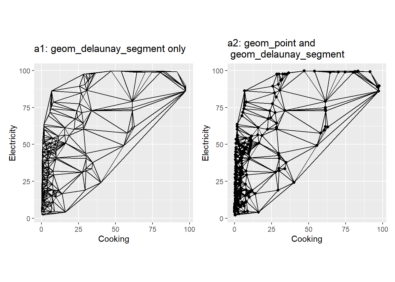
Package
ggforce (Pedersen 2022)
Description
Display voronoi tesselation and delaunay triangulation.
Understandable aesthetics
required aesthetics
x or y
optional aesthetics
alpha, colour, fill , linetype, size
See also
Example
library(ggforce)
library(deldir) #to calculate delaunay triangulation

a1 <- worldbankdata |>
  filter(Income == "L") |>
  ggplot(aes(x=Cooking, y=Electricity)) +
  geom_delaunay_segment2() +
  theme(aspect.ratio = 1) +
  labs(title = "a1: geom_delaunay_segment2 only")

a2 <- worldbankdata |>
  filter(Income == "L") |>
  ggplot(aes(x=Cooking, y=Electricity)) +
  geom_point() +
  geom_delaunay_segment2() +
  theme(aspect.ratio = 1) +
  labs(title = "a2: geom_point and \n geom_delaunay_segment2")

a1 | a2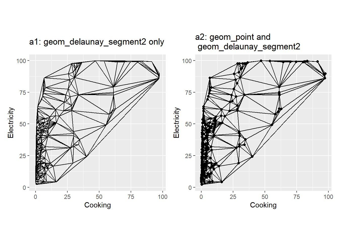
Package
ggalt(Rudis, Bolker, and Schulz 2017)
Description
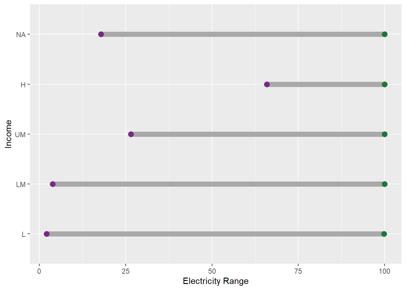
Create dumbbell charts.
Understandable aesthetics
required aesthetics
x, y, xend, yend
optional aesthetics
alpha, colour, group, linetype, size
See also
Example
library(ggalt)
df <- worldbankdata |>
  group_by(Income) |>
  summarise(min = min(Electricity, na.rm=TRUE), max = max(Electricity, na.rm=TRUE))
df
# A tibble: 5 × 3
Income min max
<fct> <dbl> <dbl>
1 L 2.11 99.8
2 LM 3.81 100
3 UM 26.5 100
4 H 65.9 100
5 <NA> 17.8 100 ggplot(df, aes(y=Income, x=min, xend=max)) +
xlab("Electricity Range") +
geom_dumbbell(color = "darkgray", # Color of the line between min and max
size = 3, # Line width
dot_guide = FALSE, # Whether to add a guide from origin to X or not
size_x = 3, # Size of the X point
size_xend = 3, # Size of the X end point
colour_x = "#762a83", # Color of the X point
colour_xend = "#1b7837") # Color of the X end point