20  geom_t

20.1 geom_text

Package

ggplot2 (Wickham 2016)

Description

Labeling plots.

Understandable aesthetics

required aesthetics

x, y

optional aesthetics

stat , position , size

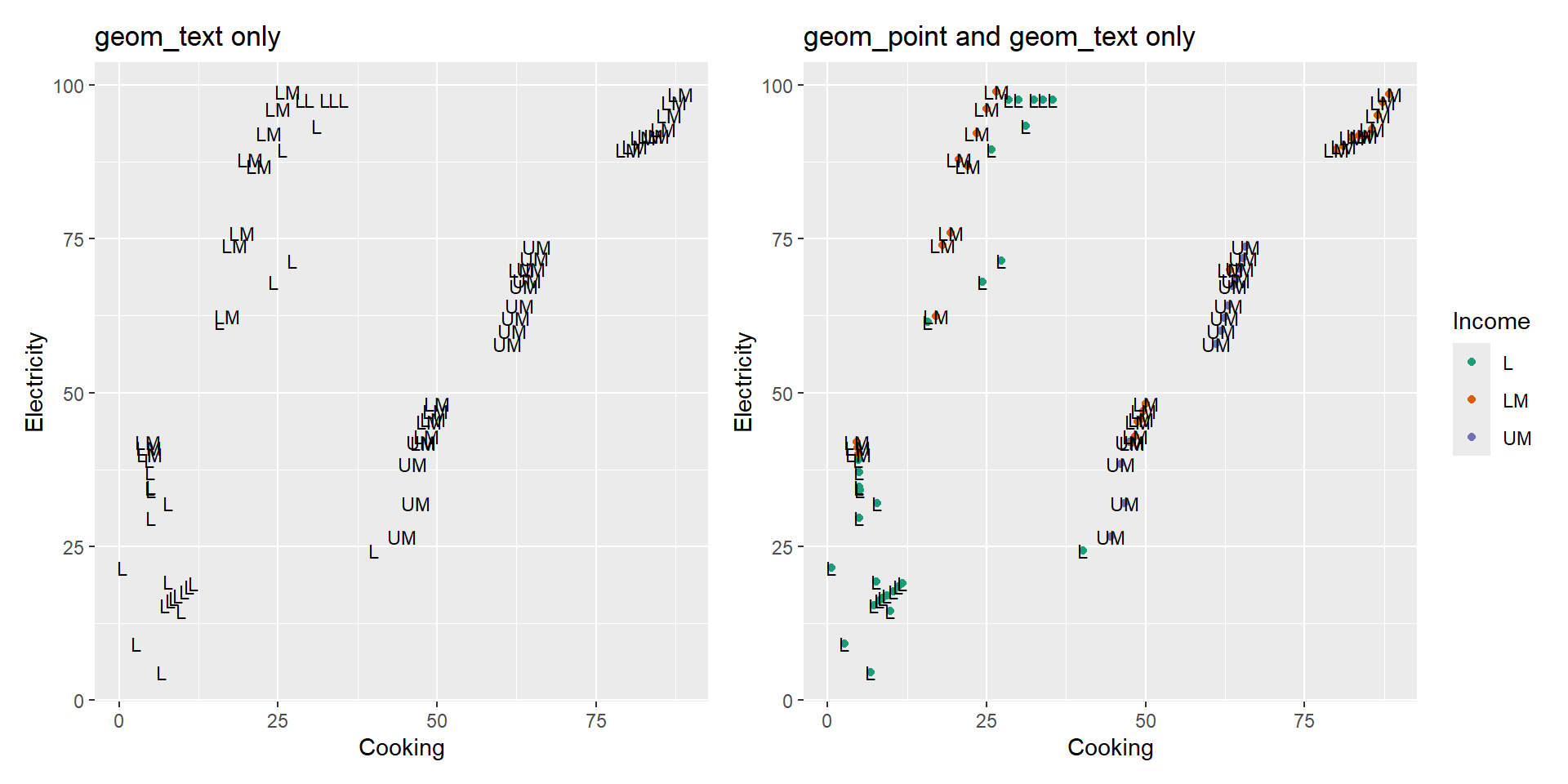
Example

p1 <- drop_na(worldbankdata) |>
  filter(Code %in% c('AFG', 'AGO', 'BEN', 'BFA', 'BGD', 'BOL', 'BWA')) |>
  ggplot(aes(x = Cooking, y = Electricity, label = Income)) + geom_text(size = 3) + scale_color_brewer(palette = "Dark2") + scale_fill_brewer(palette = "Dark2") + ggtitle("geom_text only")
p2 <- drop_na(worldbankdata) |>
  filter(Code %in% c('AFG', 'AGO', 'BEN', 'BFA', 'BGD', 'BOL', 'BWA')) |>
  ggplot(aes(x = Cooking, y = Electricity, label = Income)) + 
  geom_point(aes(color = Income)) +
  geom_text(size = 3) + scale_color_brewer(palette = "Dark2") + scale_fill_brewer(palette = "Dark2") + ggtitle("geom_point and geom_text only")
p1|p2

20.2 geom_text_repel

Package

ggrepel (Slowikowski 2024)

Description

Repulsive textual annotations.

Understandable aesthetics

required aesthetics

`x, y

optional aesthetics

stat , position , size

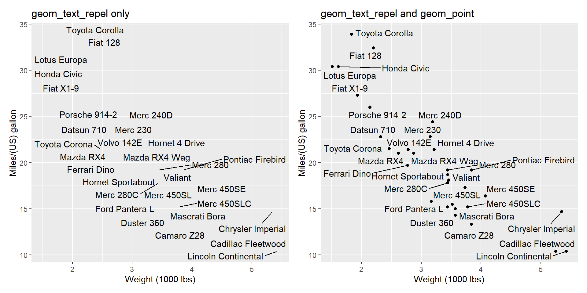
Example

library(ggrepel)
p1 <- ggplot(mtcars, aes(x = wt, y = mpg, label = rownames(mtcars))) +
  geom_text_repel() +  
  labs(title = "",x = "Weight (1000 lbs)", y = "Miles/(US) gallon") + scale_color_brewer(palette = "Dark2") + scale_fill_brewer(palette = "Dark2") + ggtitle("geom_text_repel only")
p2 <- ggplot(mtcars, aes(x = wt, y = mpg, label = rownames(mtcars))) +
  geom_point() +
  geom_text_repel() +  
  labs(title = "",x = "Weight (1000 lbs)", y = "Miles/(US) gallon") + scale_color_brewer(palette = "Dark2") + scale_fill_brewer(palette = "Dark2") + ggtitle("geom_text_repel and geom_point")
p1|p2

20.3 geom_tile

Package

ggplot2 (Wickham 2016)

Description

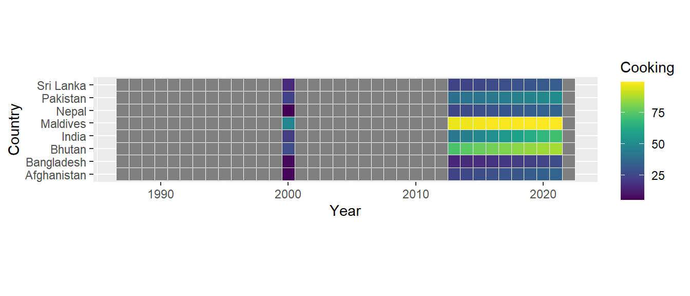
Create heat map plot. geom_rect() and geom_tile() do the same thing, but function inputs are different: geom_rect() uses the locations of the four corners (xmin, xmax, ymin and ymax), while geom_tile() uses the center of the tile and its dimensions (x, y, width, height).

Understandable aesthetics

required aesthetics

x

y

optional aesthetics

alpha, colour, group, linetype, linewidth

See also

geom_rect, geom_raster

Example

 worldbankdata |>
  filter(Region == "South Asia" ) |>
  ggplot(aes(x=Year,
             y=Country, fill=Cooking)) +
  geom_tile(aes(width=1, height=1), col="white") +
  viridis::scale_fill_viridis() +
  coord_fixed()

20.4 geom_text_cooks

Package

ggxmean (Reynolds 2024)

Description

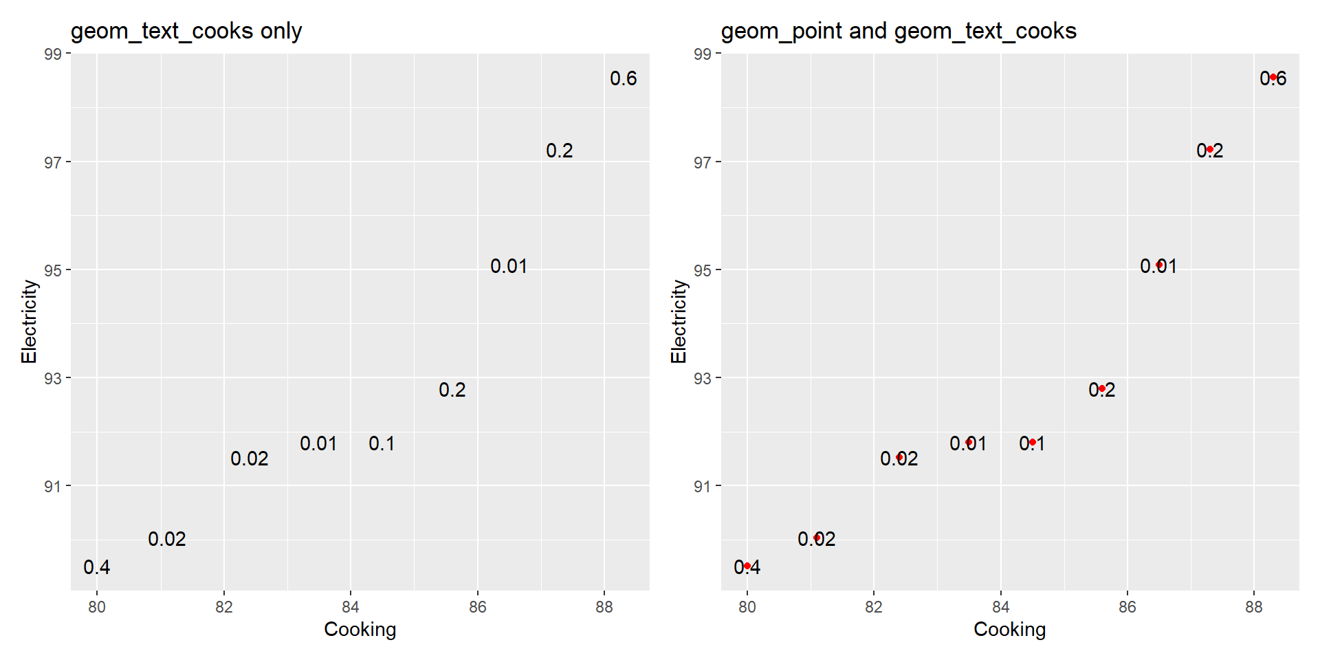
Returns a scatter plot with points that are labeled.

Understandable aesthetics

required aesthetics

x, y

optional aesthetics

position , size, digits, check_overlap

See also

geom_scatter, geom_text, geom_label

Example

library(ggxmean)
p1 <- worldbankdata |>
  filter(Country == "Bolivia" & Cooking > 75) |>
  ggplot(aes(x=Cooking, y=Electricity)) + 
  geom_text_cooks(check_overlap = TRUE, digits = 1) + ggtitle("geom_text_cooks only")  
p2 <- worldbankdata |>
  filter(Country == "Bolivia" & Cooking > 75) |>
  ggplot(aes(x=Cooking, y=Electricity)) + 
  geom_point(col="red") +
  geom_text_cooks(check_overlap = TRUE, digits = 1) + ggtitle("geom_point and geom_text_cooks") 
p1|p2

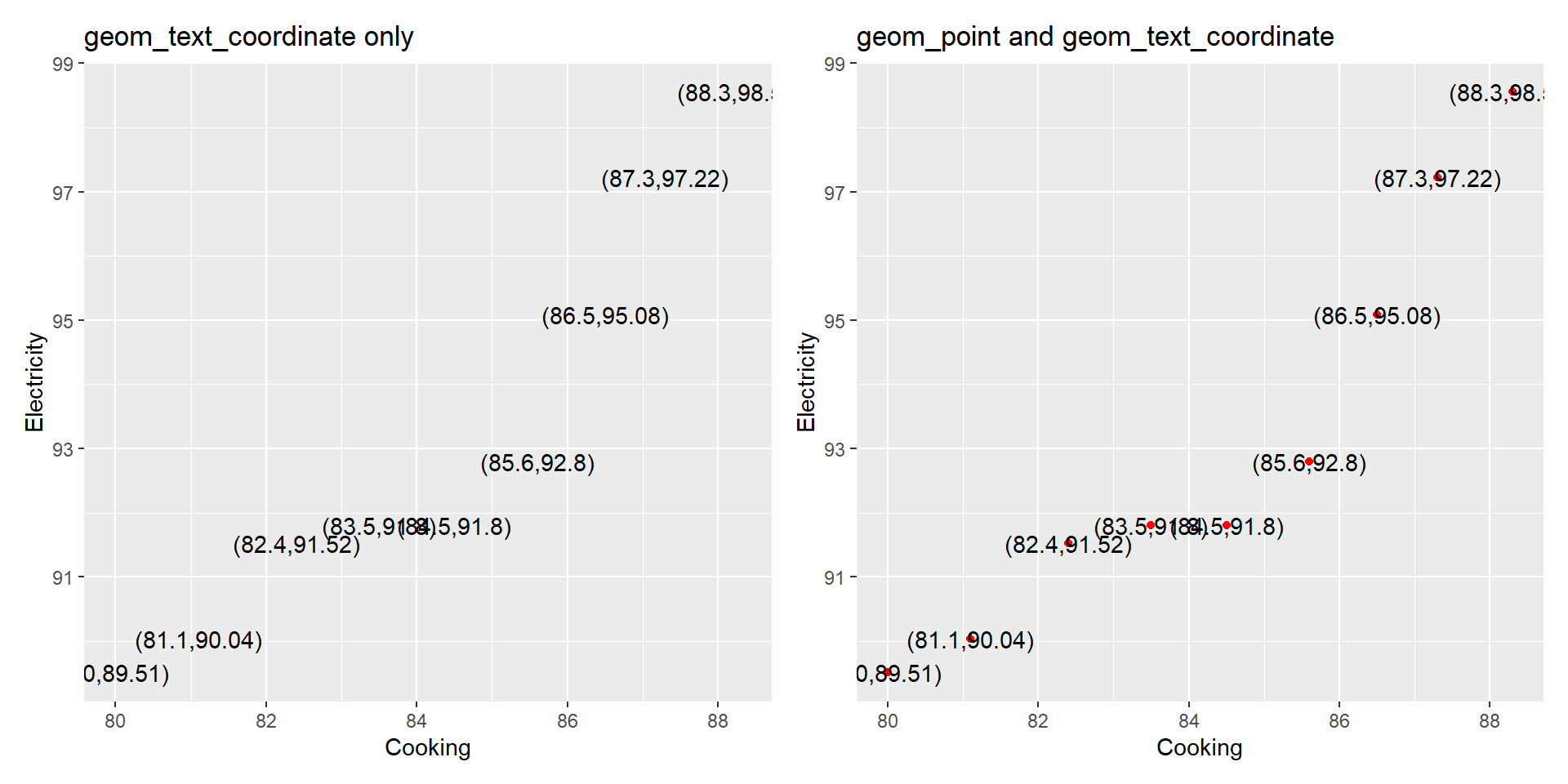
20.5 geom_text_coordinate

Package

ggplot2 (Wickham 2016)

Description

Returns a scatter plot with points that are labeled with (x, y) coordinates.

Understandable aesthetics

required aesthetics

x

y

optional aesthetics

position, size, check_overlap, nudge_x

See also

geom_text, geom_text_cooks, geom_text_repel

Example

p1 <- worldbankdata |>
  filter(Country == "Bolivia" & Cooking > 75) |>
  ggplot(aes(x=Cooking, y=Electricity)) + 
  geom_text_coordinate() +
  ggtitle("geom_text_coordinate only")

p2 <- worldbankdata |>
  filter(Country == "Bolivia" & Cooking > 75) |>
  ggplot(aes(x=Cooking, y=Electricity)) + 
  geom_point(col="red") +
  geom_text_coordinate() +
  ggtitle("geom_point and geom_text_coordinate")
p1|p2

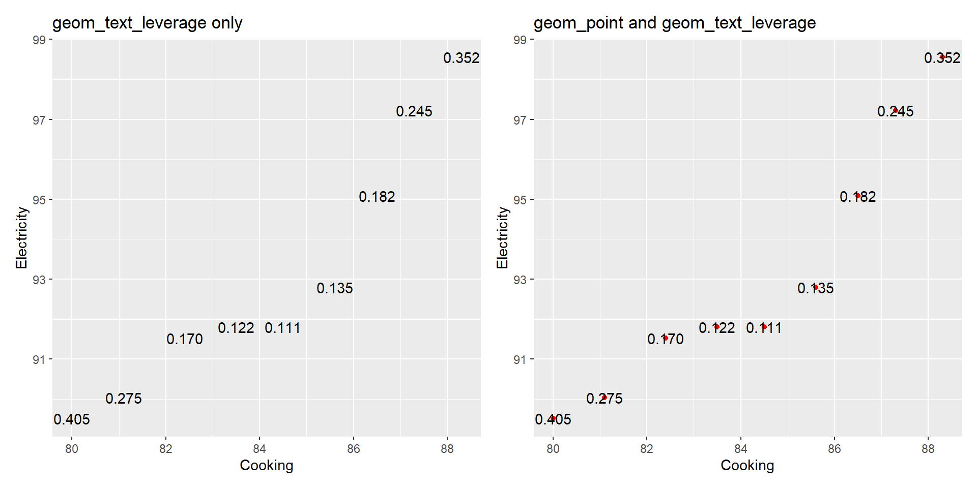
20.6 geom_text_leverage

Package

ggxmean (Reynolds 2024)

Description

Returns a scatter plot with points that are labeled.

Understandable aesthetics

required aesthetics

x, y

optional aesthetics

position , size, check_overlap, nudge_x

See also

geom_text, geom_text_cooks, geom_text_repel

Example

p1 <- worldbankdata |>
  filter(Country == "Bolivia" & Cooking > 75) |>
  ggplot(aes(x=Cooking, y=Electricity)) + 
  geom_text_leverage() +
  ggtitle("geom_text_leverage only")

p2 <- worldbankdata |>
  filter(Country == "Bolivia" & Cooking > 75) |>
  ggplot(aes(x=Cooking, y=Electricity)) + 
  geom_point(col="red") +
  geom_text_leverage() +
  ggtitle("geom_point and geom_text_leverage")
p1|p2

Reynolds, Evangeline. 2024. Ggxmean: Statistical Geoms.

Slowikowski, Kamil. 2024. Ggrepel: Automatically Position Non-Overlapping Text Labels with ’Ggplot2’. https://CRAN.R-project.org/package=ggrepel.

Wickham, Hadley. 2016. Ggplot2: Elegant Graphics for Data Analysis. Springer-Verlag New York. https://ggplot2.tidyverse.org.