ggplot() +
  geom_function(fun = ~ 0.5*exp(-abs(.x)))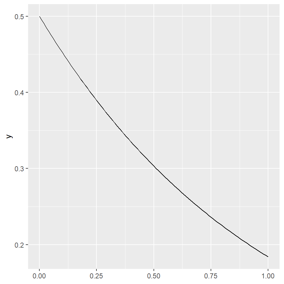
ggplot2 (Wickham 2016)
Computes and draws a function as a continuous curve.
required aesthetics
x
y
optional aesthetics
alpha, colour, group, linetype, linewidth
stat_prefix
ggplot() +
geom_function(fun = ~ 0.5*exp(-abs(.x)))
ggplot2 (Wickham 2016)
Visualise the spread of a single continuous variable by partitioning the x-axis into bins and mapping the frequency of observations within each bin.
required aesthetics
x
y
optional aesthetics
alpha, colour, group, linetype, linewidth
stat_bin for a continuous x variable
stat_count for a discrete x variable
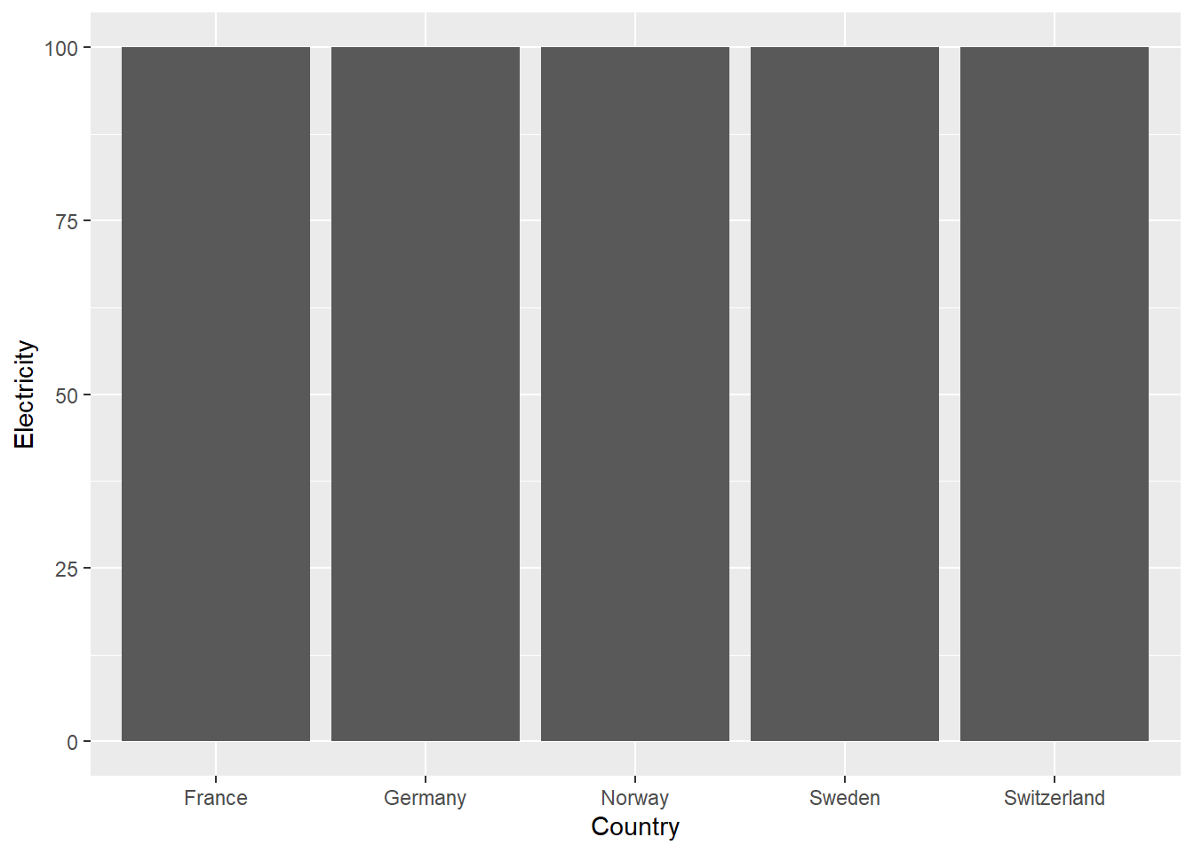
worldbankdata |>
  ggplot(aes(x=Electricity, col=Income)) +
  geom_freqpoly()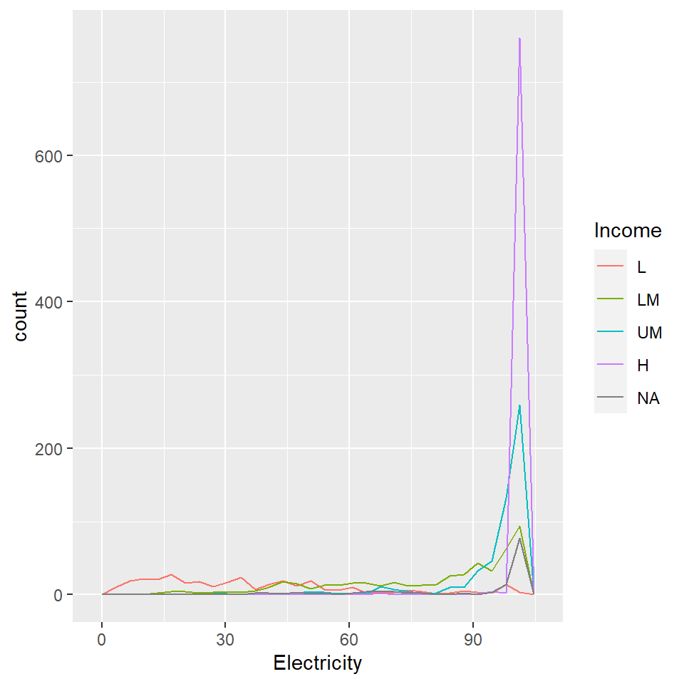
library(ggimage)
worldbankdata.flag <- worldbankdata |>
  filter(Country %in% c("France", "Sweden", "Norway", "Germany", "Switzerland")) |>
  filter(Year == 2000)
worldbankdata.flag$code.flag <- c("FR", "SE", "NO", "DE", "CH")
worldbankdata.flag |>
ggplot(aes(y = Country, x= Electricity)) +
  geom_col(stat = 'identity') +
  geom_flag(y = -2, aes(image = code.flag)) +
  coord_flip()