19 S

19.1 geom_smooth

Package

ggplot2 (Wickham 2016)

Description

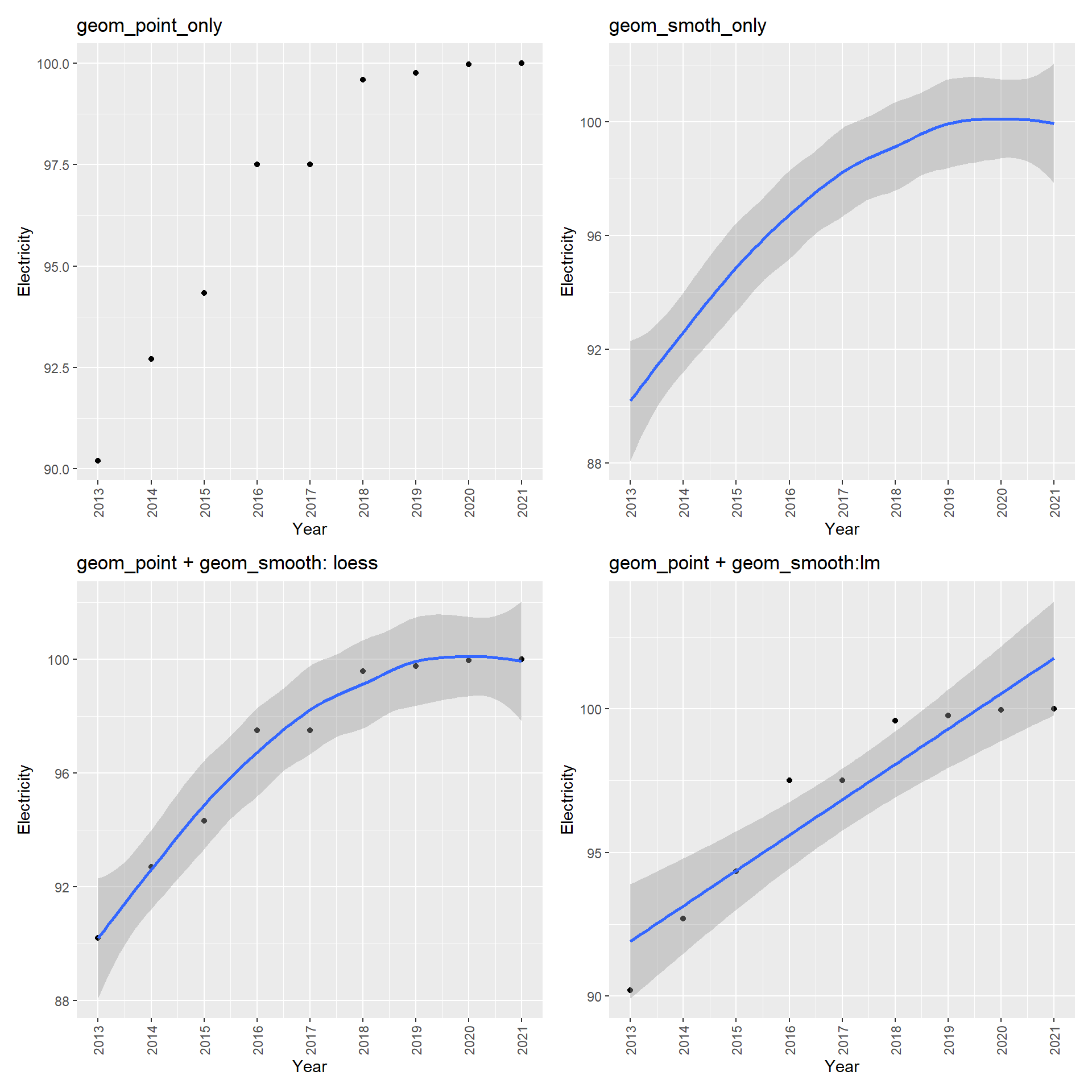
Add a smooth curve or line to a scatter plot for visulizing trend between x and y variable.

See also

geom_point

Understandable aesthetics

Required aesthetics
- x, y
Optional aesthetics
- alpha, colour, fill, group, linetype, linewidth, weight, ymax, ymin

The statistical transformation to use on the data for this layer

smooth

Example

p1 <- worldbankdata |>
  filter(Country == "Sri Lanka" ) |>
  filter(Year >= 2013 & Year <= 2021) |> 
  ggplot(aes(x=Year, y=Electricity)) + 
  geom_point() +
  theme(axis.text.x = element_text(angle = 90, vjust = 0.5, hjust=1)) + 
  scale_x_continuous(breaks = 2000:2021)  + 

  ggtitle("geom_point_only")

p2 <- worldbankdata |> 
  filter(Country == "Sri Lanka" ) |>
  filter(Year >= 2013 & Year <= 2021) |>
  ggplot(aes(x=Year, y=Electricity)) + 
  geom_smooth() +
  theme(axis.text.x = element_text(angle = 90, vjust = 0.5, hjust=1)) + 
  scale_x_continuous(breaks = 2000:2021)  + 
  ggtitle("geom_smoth_only")

p3 <- worldbankdata |>
  filter(Country == "Sri Lanka" ) |> 
  filter(Year >= 2013 & Year <= 2021) |>
  ggplot(aes(x=Year, y=Electricity)) + 
  geom_point() +
  geom_smooth() +
  theme(axis.text.x = element_text(angle = 90, vjust = 0.5, hjust=1)) + 
  scale_x_continuous(breaks = 2000:2021)  + 
  ggtitle("geom_point + geom_smooth: loess")

p4 <- worldbankdata |> 
  filter(Country == "Sri Lanka" ) |>
  filter(Year >= 2013 & Year <= 2021) |> 
  ggplot(aes(x=Year, y=Electricity)) + 
  geom_point() +
  geom_smooth(method = "lm") +
  theme(axis.text.x = element_text(angle = 90, vjust = 0.5, hjust=1)) + 
  scale_x_continuous(breaks = 2000:2021)  + 
  ggtitle("geom_point + geom_smooth:lm")

(p1 + p2)/(p3+p4)

19.2 geom_segment

Package

ggplot2 (Wickham 2016)

Description

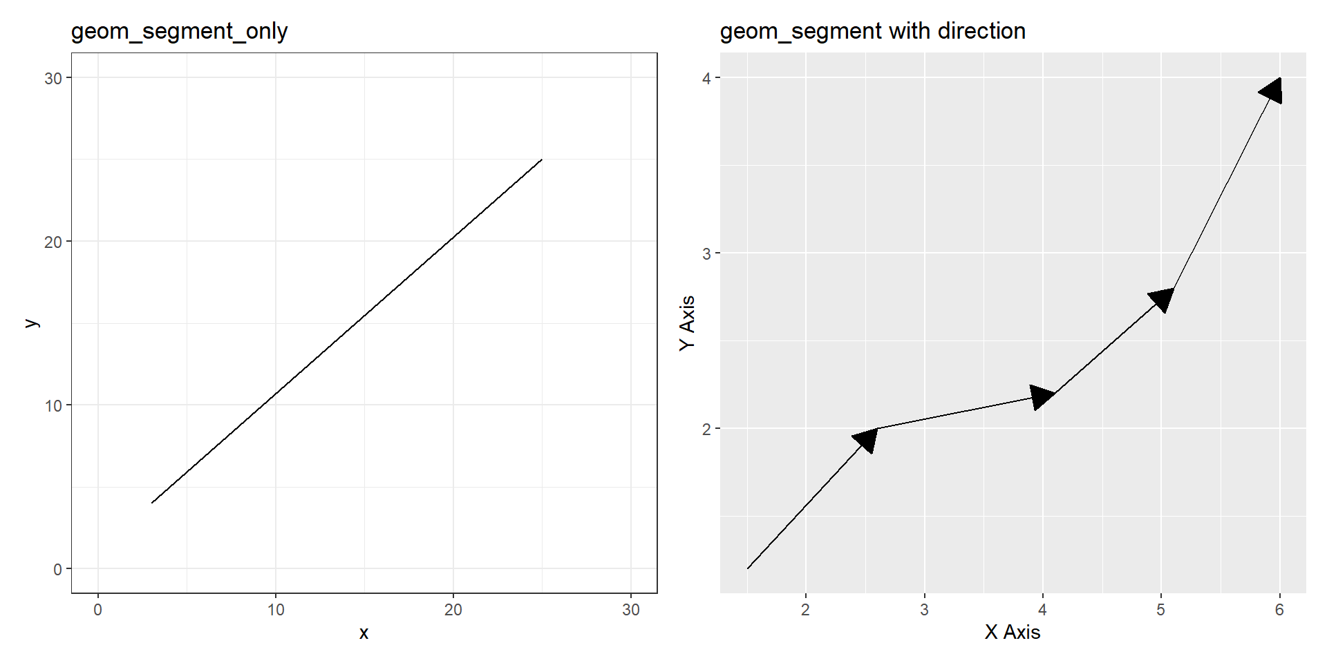
Add a straight line segment between two points.

Understandable aesthetics

Required aesthetics
- x, y, xend or yend
Optional aesthetics
- alpha, colour, group, linetype, linewidth

The statistical transformation to use on the data for this layer

identity

See Also

geom_curve(), geom_path(), geom_line(), geom_spoke()

Examples

Example 1: simulated data

p1 <- ggplot() + 
  geom_segment(aes(x = 3, y = 4, xend = 25, yend = 25)) +
  theme_minimal() +
  coord_cartesian(ylim = c(0, 30), xlim = c(0, 30)) +
  theme_bw()+
  ggtitle("geom_segment_only")


data <- data.frame(
  x_start = c(1.5, 2.6, 4.1, 5.1),
  y_start = c(1.2, 2, 2.2, 2.8),
  x_end = c(2.6, 4.1, 5.1, 6),
  y_end = c(2, 2.2, 2.8, 4))

p2 <- ggplot(data) +
  geom_segment(aes(x = x_start, y = y_start, xend = x_end, yend = y_end),
               color = "black", size = 0.5, 
               arrow = arrow(type = "closed", length = unit(0.2, "inches"))) +
  labs(x = "X Axis",
       y = "Y Axis") +
  ggtitle("geom_segment with direction")
p1+p2

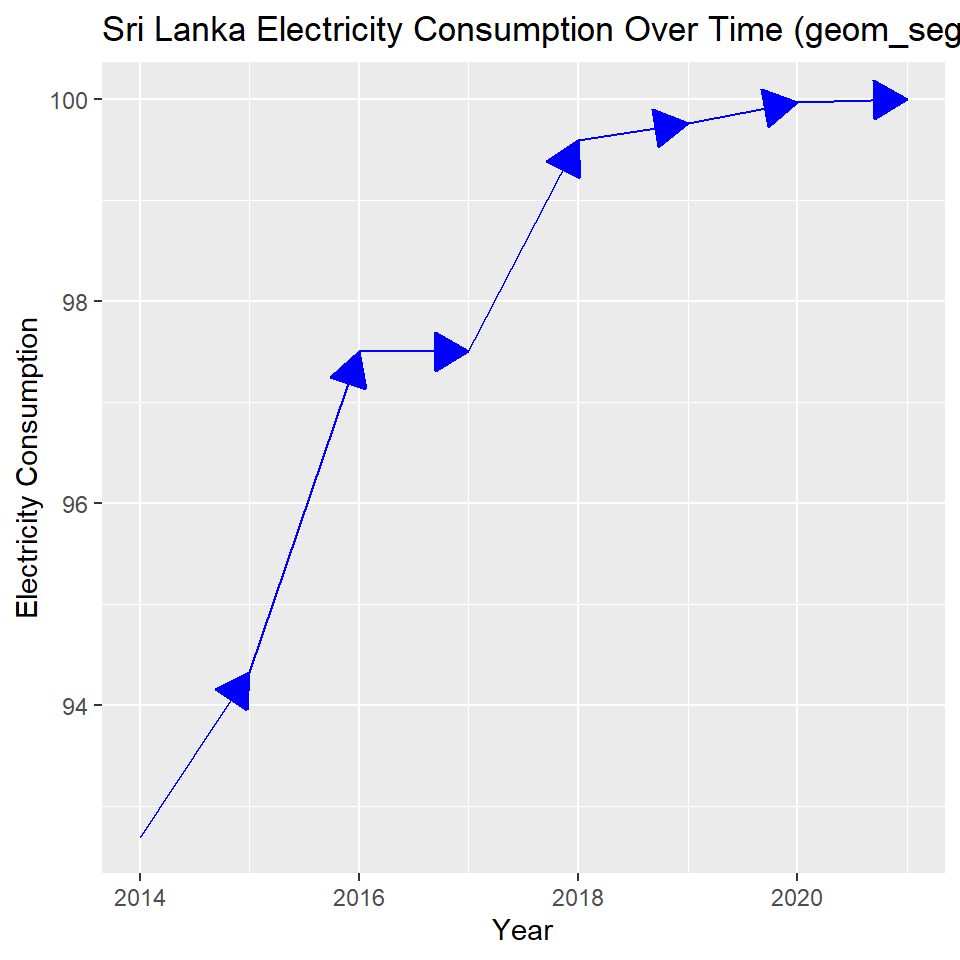
Example 2: Application data

SL_segments <- worldbankdata |> 
  filter(Country == "Sri Lanka" & Year > 2013) |> 
     mutate(
    x_end = lead(Year), 
    y_end = lead(Electricity)  
  ) |> 
  filter(!is.na(x_end) & !is.na(y_end))

 ggplot(SL_segments) +
  geom_segment(aes(x = Year, y = Electricity, xend = x_end, 
                   yend = y_end),
               color = "blue", size = 0.5, arrow = arrow(type = "closed", length = unit(0.2, "inches"))) +
  labs(x = "Year",
       y = "Electricity Consumption",
       title = "Sri Lanka Electricity Consumption Over Time (geom_segment)")

19.3 geom_spoke

Package

ggplot2 (Wickham 2016)

Description

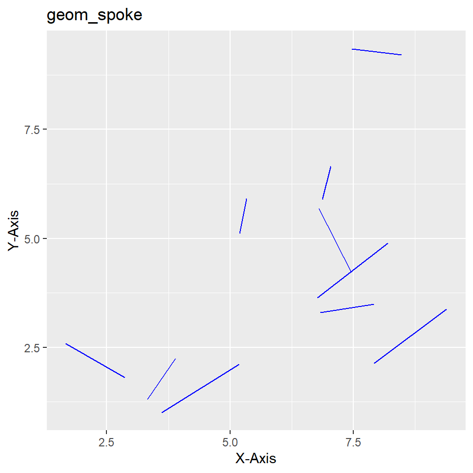
Creates radial line segments (spokes) from a central point, where each spoke is defined by its angle and radius. This is useful for visualizing directions or vectors.

Understandable aesthetics

Required aesthetics
- x, y, angle, radius
Optional aesthetics
- alpha, colour, group, linetype, linewidth

The statistical transformation to use on the data for this layer

identity

Examples

Example: Simulated data

set.seed(8)
data <- tibble(
  x = runif(10, 1, 10),      # Random x-coordinates
  y = runif(10, 1, 10),      # Random y-coordinates
  angle = runif(10, 0, 2 * pi),  # Random angles in radians
  radius = runif(10, 0.5, 2) # Random lengths for spokes
)


ggplot(data, aes(x = x, y = y)) +
  geom_spoke(aes(angle = angle, radius = radius),
             color = "blue", size = 0.5) +
  labs(x = "X-Axis", 
       y = "Y-Axis", 
       title = "geom_spoke")

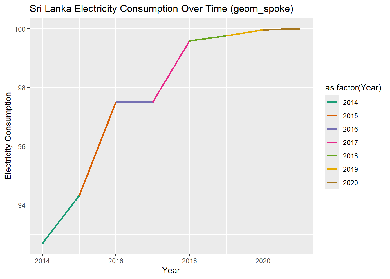
Example: Practical application data

SL <- worldbankdata |> 
  filter(Country == "Sri Lanka" & Year > 2013)

# Prepare the data for geom_spoke
SL_segments <- SL |> 
  mutate(
    x_end = lead(Year),  # Next year
    y_end = lead(Electricity)  # Next year's electricity value
  ) |> 
  filter(!is.na(x_end) & !is.na(y_end)) |> 
  mutate(
    angle = atan2(y_end - Electricity, x_end - Year),  # Angle in radians
    radius = sqrt((x_end - Year)^2 + (y_end - Electricity)^2)  # Euclidean distance
  )

# Plot with geom_spoke
ggplot(SL_segments, aes(x = Year, y = Electricity, color=as.factor(Year))) +
  geom_spoke(aes(angle = angle, radius = radius), size = 1) +
  scale_color_brewer(type = "qual", palette = 2) +
  labs(x = "Year",
       y = "Electricity Consumption",
       title = "Sri Lanka Electricity Consumption Over Time (geom_spoke)")

19.4 geom_step

Package

ggplot2 (Wickham 2016)

Description

Create stairstep plot: Connect observations in the order in which they appear in the data by stairs.

Understandable aesthetics

Required aesthetics
- x, y
Optional aesthetics
- alpha, colour, group, linetype, linewidth

The statistical transformation to use on the data for this layer

identity

See Also

geom_path(), geom_line(), geom_polygon(), geom_segment()

Example

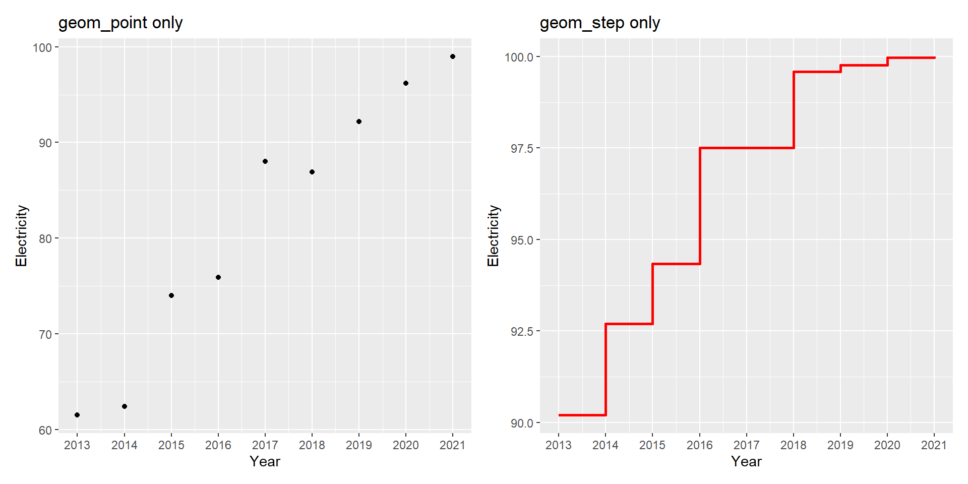
p1 <- worldbankdata |> 
  filter(Country == "Bangladesh") |>
  filter(Year >= 2013 & Year <= 2021) |>
  ggplot(aes(x=Year, y=Electricity)) + 
  geom_point() + 
  scale_x_continuous(breaks = 2013:2021)  + 
  ggtitle("geom_point only")

p2 <- worldbankdata |> 
  filter(Country == "Sri Lanka") |>
  filter(Year >= 2013 & Year <= 2021) |>
  ggplot(aes(x=Year, y=Electricity)) + 
  geom_step(color = "red", size = 1) + 
  scale_x_continuous(breaks = 2013:2021)  + 
  ggtitle("geom_step only")

p1 + p2

19.5 geom_sf

Package

ggplot2 (Wickham 2016)

Description

Visualize sf objects.

Understandable aesthetics

Required aesthetics
- simple feature geometry
Optional aesthetics
- alpha, colour, group, fill

The statistical transformation to use on the data for this layer

See Also

geom_sf_label(), geom_sf_text()

Example

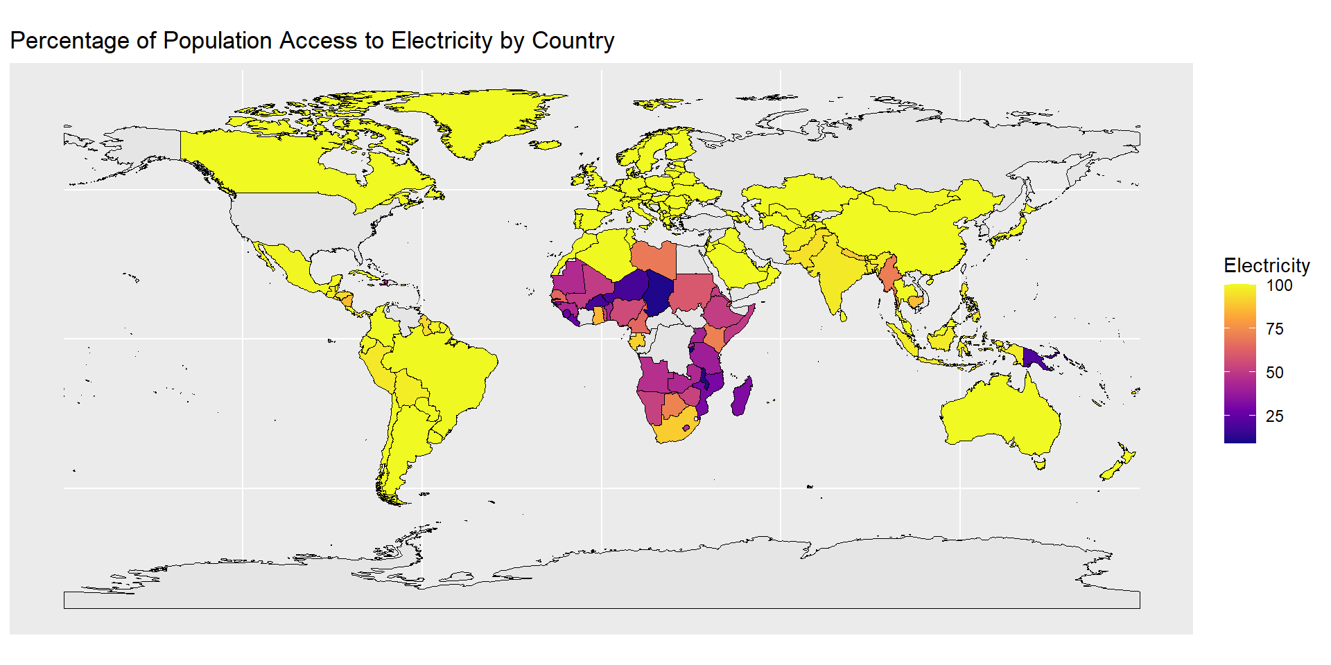
library(rnaturalearth)
library(rnaturalearthdata)

# Load world spatial data
world <- ne_countries(scale = "medium", returnclass = "sf")

electricity_data <- worldbankdata |> filter(Year == 2020)
world_electricity <- world |> 
  left_join(electricity_data, by = c("name" = "Country"))

ggplot(data = world_electricity) +
  geom_sf(aes(fill = Electricity), color = "black", size = 0.1) +
  scale_fill_viridis_c(option = "plasma", na.value = "grey90") +
  labs(
    title = "Percentage of Population Access to Electricity by Country",
    fill = "Electricity")

19.6 geom_sf_label

Package

ggsflabel (Yutani 2024)

# install.packages("devtools")
devtools::install_github("yutannihilation/ggsflabel")

Description

Add text labels to spatial features in a plot created with geom_sf()

Understandable aesthetics

Required aesthetics
- label
Optional aesthetics
- alpha, colour, group, fill

The statistical transformation to use on the data for this layer

sf_coordinates

See Also

geom_sf(), geom_sf_text()

Example

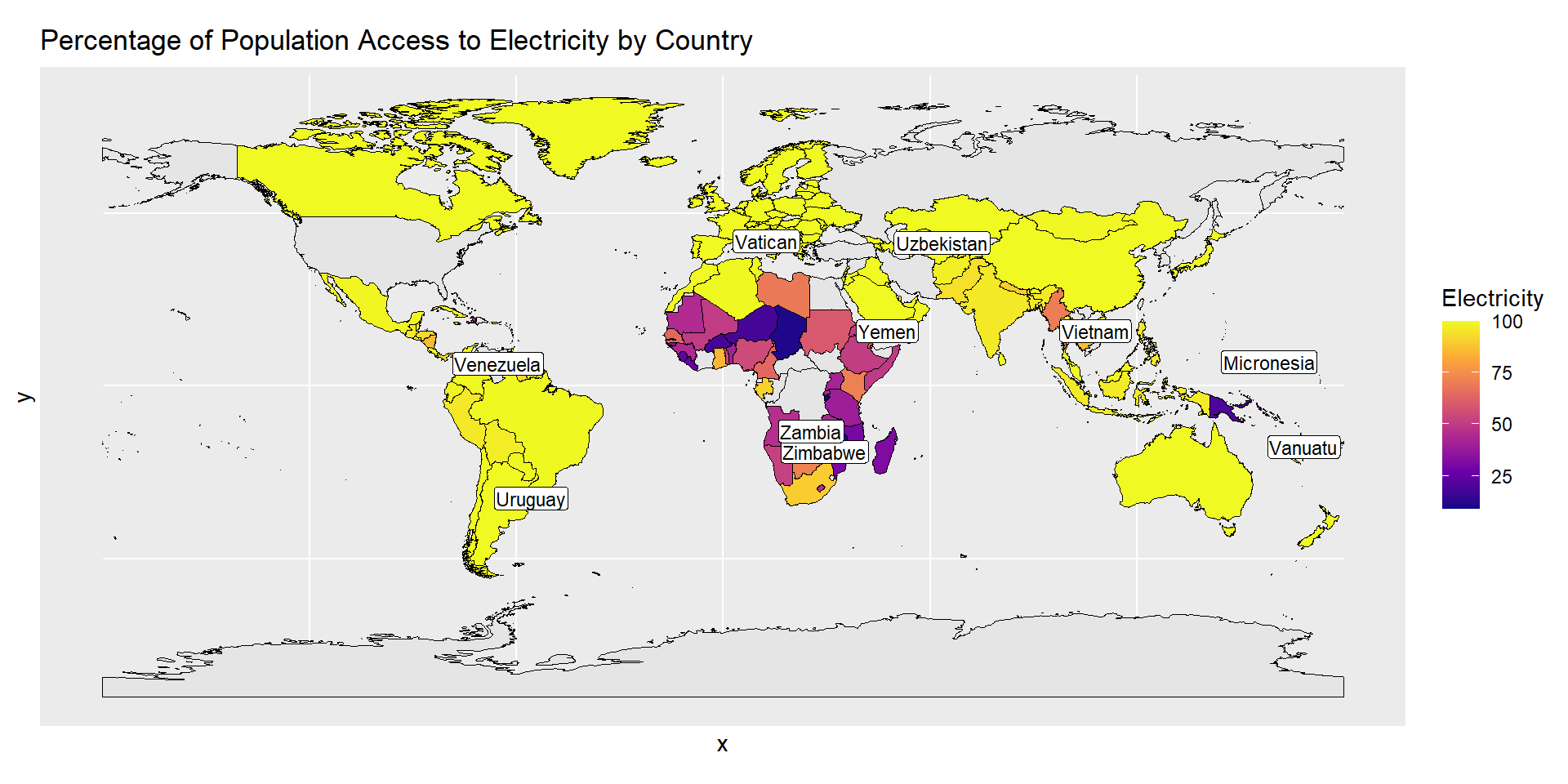
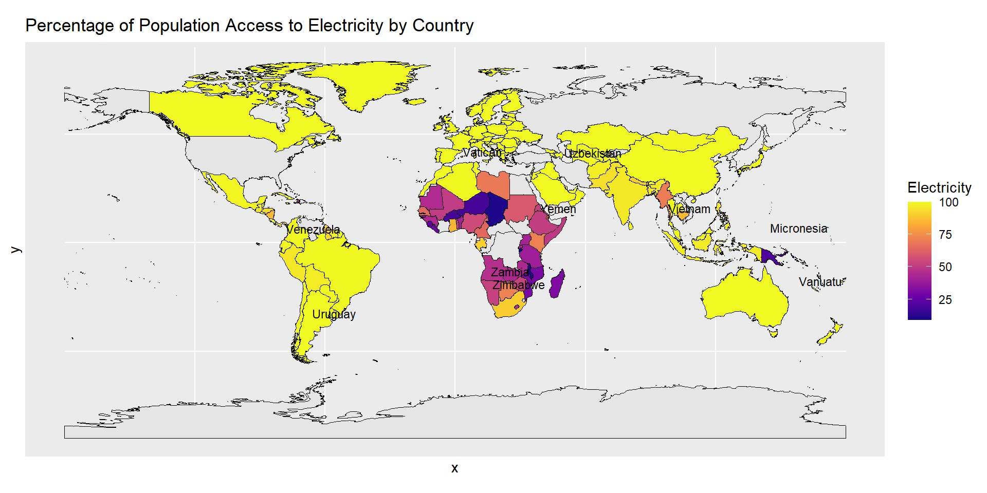
library(rnaturalearth)
library(rnaturalearthdata)

# Load world spatial data
world <- ne_countries(scale = "medium", returnclass = "sf")

electricity_data <- worldbankdata |> filter(Year == 2020)
world_electricity <- world |> 
  left_join(electricity_data, by = c("name" = "Country"))

countries_to_label <- world_electricity |> head(10)

ggplot(data = world_electricity) +
  geom_sf(aes(fill = Electricity), color = "black", size = 0.1) +
   geom_sf_label(data = countries_to_label, aes(label = name), size = 3, label.padding = unit(0.1, "lines")) +
  scale_fill_viridis_c(option = "plasma", na.value = "grey90") +
  labs(
    title = "Percentage of Population Access to Electricity by Country",
    fill = "Electricity")

19.7 geom_sf_text

ggsflabel (Yutani 2024)

# install.packages("devtools")
devtools::install_github("yutannihilation/ggsflabel")

Description

Add text labels to spatial features in a plot created with geom_sf() without the background box. It is a similar approach as with geom_sf_label().

Understandable aesthetics

Required aesthetics
- label
Optional aesthetics
- alpha, colour, group, fill

The statistical transformation to use on the data for this layer

sf_coordinates

See Also

geom_sf(), geom_sf_label()

Example

library(rnaturalearth)
library(rnaturalearthdata)

# Load world spatial data
world <- ne_countries(scale = "medium", returnclass = "sf")

electricity_data <- worldbankdata |> filter("Year" == 2020 )
world_electricity <- world |> 
  left_join(electricity_data, by = c("name" = "Country"))

countries_to_label <- world_electricity |> head(10)

ggplot(data = world_electricity) +
  geom_sf(aes(fill = Electricity), color = "black", size = 0.1) +
   geom_sf_text(data = countries_to_label, aes(label = name), size = 3, label.padding = unit(0.1, "lines")) +
  scale_fill_viridis_c(option = "plasma", na.value = "grey90") +
  labs(
    title = "Percentage of Population Access to Electricity by Country",
    fill = "Electricity")

19.8 geom_sf_pattern

Package

ggpattern (FC, Davis, and ggplot2 authors 2023)

Description

Add patterns to the map.

Understandable aesthetics

Required aesthetics
- NuULL
Optional aesthetics
- alpha, colour, group, fill

The statistical transformation to use on the data for this layer

sf_coordinates

Example

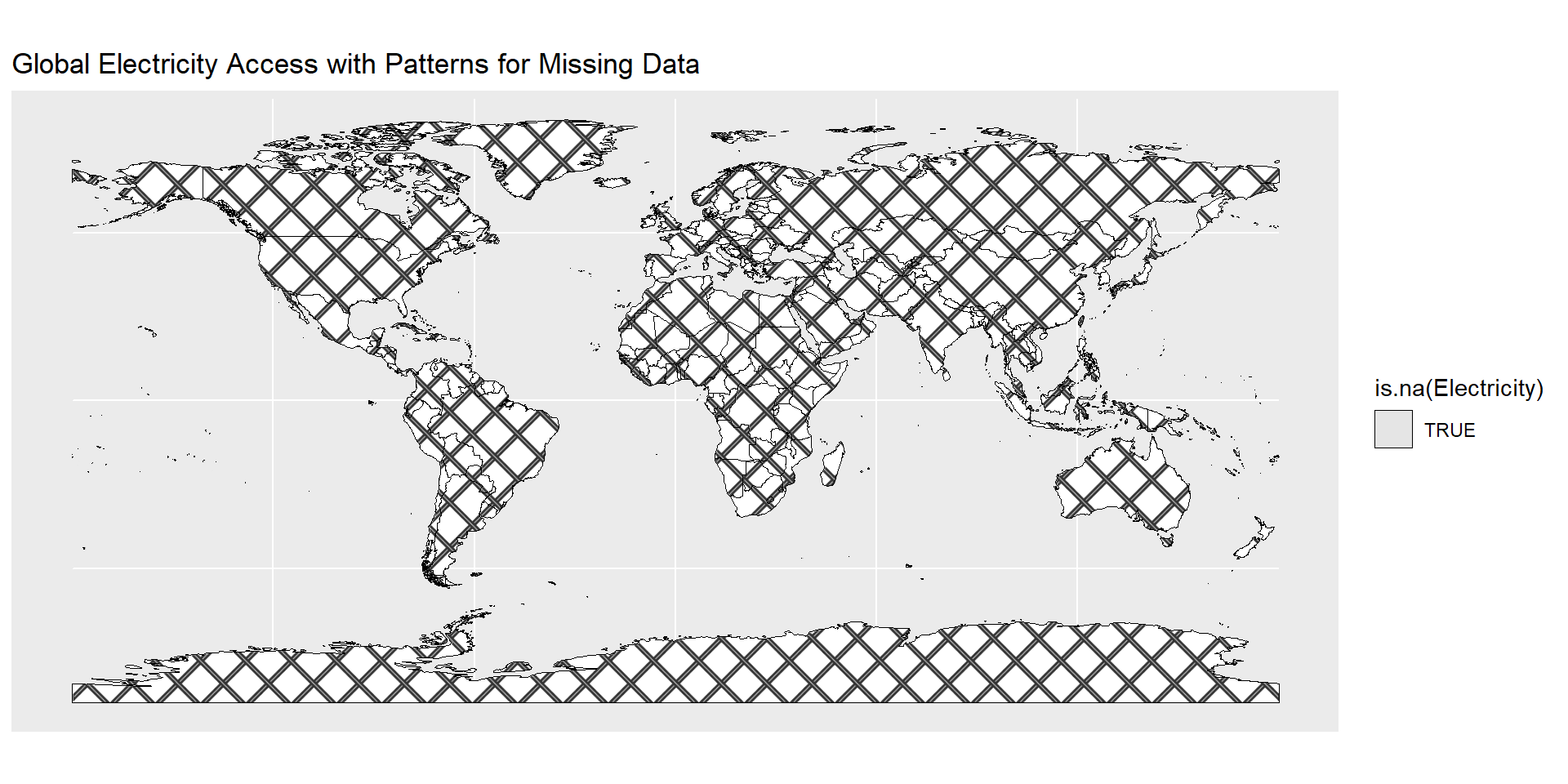
library(rnaturalearth)
library(rnaturalearthdata)
library(ggpattern)

# Load world spatial data
world <- ne_countries(scale = "medium", returnclass = "sf")

electricity_data <- worldbankdata |> filter("Year" == 2020)
world_electricity <- world |> 
  left_join(electricity_data, by = c("name" = "Country"))

ggplot(data = world_electricity) +
  geom_sf_pattern(aes(fill = Electricity, pattern = is.na(Electricity)), 
                  color = "black", 
                  size = 0.1,
                  pattern_fill = "gray80", 
                  pattern_angle = 45, 
                  pattern_density = 0.1) +
  scale_fill_viridis_c(option = "plasma", na.value = "white") +
  labs(
    title = "Global Electricity Access with Patterns for Missing Data",
    fill = "Electricity (GWh)"
  )

FC, Mike, Trevor L Davis, and ggplot2 authors. 2023. Ggpattern: ’Ggplot2’ Pattern Geoms.

Wickham, Hadley. 2016. Ggplot2: Elegant Graphics for Data Analysis. Springer-Verlag New York. https://ggplot2.tidyverse.org.

Yutani, Hiroaki. 2024. Ggsflabel: Labels for ’Sf’ with ’Ggplot2’. https://github.com/yutannihilation/ggsflabel.